Accurate Bathymetric Maps From Underwater Digital Imagery Without Ground Control

Introduction

Benthic ecosystems throughout the world have been stressed by human impacts, including land-based pollution, overharvesting, coastal engineering, ocean acidification, and climate change (Hughes, 1994; Edinger et al., 1998; Kleypas and Yates, 2009; Storlazzi et al., 2015; Toth et al., 2015; Prouty et al., 2017; Takesue and Storlazzi, 2019). It is critical, therefore, to develop accurate geospatial inventories of benthic systems and track structural and compositional changes over time. An important element of monitoring benthic habitats is the development of accurate maps of species distribution, health, and diversity in relation to seafloor composition characteristics such as reef, rock, rubble, and sand (Burns et al., 2016; Raoult et al., 2017; Magel et al., 2019). Additionally, accurate measurements of the three-dimensional (3D) structure of reefs and changes in reef elevation over time advances understanding of reef hydrodynamics, growth, and erosion (Kuffner et al., 2019).

New opportunities to map accurately and at high resolution have been made possible by advancements in Structure-from-Motion (SfM) photogrammetry, which include feature identification and matching in photos; bundle adjustment computations of camera positions, orientations, and lens distortions; multi-view stereo techniques; GPU and network-based computing. When combined, these techniques can rapidly produce high-density, three-dimensional point clouds with associated color information from source photos (Matthews, 2008; Westoby et al., 2012; Fonstad et al., 2013). With the addition of high-quality digital cameras to novel photographing platforms including drones, and digital sources of historical photos, a resurgence of photogrammetric mapping for natural resource management has occurred during the past decade (Chirayath and Earle, 2016; Storlazzi et al., 2016; Casella et al., 2017; Pizarro et al., 2017; Warrick et al., 2017).

Structure-from-Motion photogrammetry was initially developed and applied to terrestrial settings, but it has also become an important tool for creating three dimensional models of underwater bathymetry and habitats (Li et al., 1997; Cocito et al., 2003; Burns et al., 2015, 2016; Leon et al., 2015; Storlazzi et al., 2016; Ferrari et al., 2017; Pizarro et al., 2017; House et al., 2018; Chirayath and Instrella, 2019; Price et al., 2019). In certain applications underwater SfM products have several benefits over more traditional sonar and lidar bathymetric maps. Perhaps the most important of these advantages is the incorporation of color imagery into the final products, which can be used to identify benthic features and characteristics, including substrate type and a diversity of marine species (Burns et al., 2016; Chirayath and Instrella, 2019; Magel et al., 2019). These SfM-based products also enable the development of accurate micro-roughness maps for studies of flow distribution and sediment re-suspension (Rogers et al., 2018; Pomeroy et al., 2019).

Several underwater SfM techniques exist, including photographing the seafloor from both above and below the water surface (Burns et al., 2015; Leon et al., 2015; Massot-Campos and Oliver-Codina, 2015; Chirayath and Earle, 2016; Raoult et al., 2016; Storlazzi et al., 2016; Casella et al., 2017; Pizarro et al., 2017; Raber and Schill, 2019). However, consistent with terrestrial SfM mapping, bathymetric SfM products will be optimized when best practices and accurate ancillary data are included in the workflow (Matthews, 2008). Additionally, the use of multiple cameras with different perspectives can increase the likelihood of obtaining accurate photogrammetry products (Raber and Schill, 2019). Notable factors for optimizing SfM workflows include: a stable camera and lens that can be accurately modeled by lens calibration equations; adequate photograph resolution, clarity, and overlap geometry; and high-accuracy photo positions and/or ground control, which can be used to scale and georeference SfM products (Matthews, 2008; Pizarro et al., 2017). Applied to underwater SfM, these best practices include the use of a camera with a global (not rolling) shutter, a fixed lens with constant aperture and focus settings, a lens and sensor with geometries that are not affected by camera power cycles, underwater housings that – when combined with the camera system – can be adequately modeled by lens calibration equations, adequate spatial distribution of seafloor ground control with surveyed coordinates, and accurate camera positions for each photo. Unfortunately, it can be difficult to develop an underwater ground control network for seafloor settings owing to the challenge of deploying and accurately surveying a proper constellation of markers (Casella et al., 2017; Neyer et al., 2018). These difficulties have made accurately scaled, repeatable and georeferenced bathymetric maps largely unattainable, thereby necessitating co-registration methods to map change with SfM (Burns et al., 2015; Neyer et al., 2018; Magel et al., 2019).

Here we describe, test, and evaluate a new underwater SfM mapping system that incorporates many of the photogrammetric principles mentioned above to map shallow benthic settings, such as coral reefs, without surveyed ground control points. Important elements of this system include: integration of multiple cameras and a survey-grade Global Navigation Satellite System (GNSS), high precision temporal coupling across all measurements, low distortion camera housings, a rigid frame to ensure constant camera-to-GNSS antenna geometry, and a sufficiently small system to ship to remote locations and operate from small vessels. We tested this system in diverse locations of the Florida Keys Reef Tract (Figure 1) and evaluated the geospatial accuracy of SfM products by comparing with known locations of previously surveyed human-made seafloor structures visible in the SfM reconstructions and with multiple independent surveys of a single site to test repeatability. Accuracy of local small-scale measurements from the SfM maps was assessed by imaging precision-machined 3D scale bars that were temporarily placed on the seabed in the survey area. Our results were used to evaluate the quality of mapping products generated over different benthic settings, including live reef, senile reef, reef rubble, and sand. We use these results to comment on the potential application of similar systems for generating accurate high-resolution surveys of complex seafloor structure and composition and measuring changes over time.

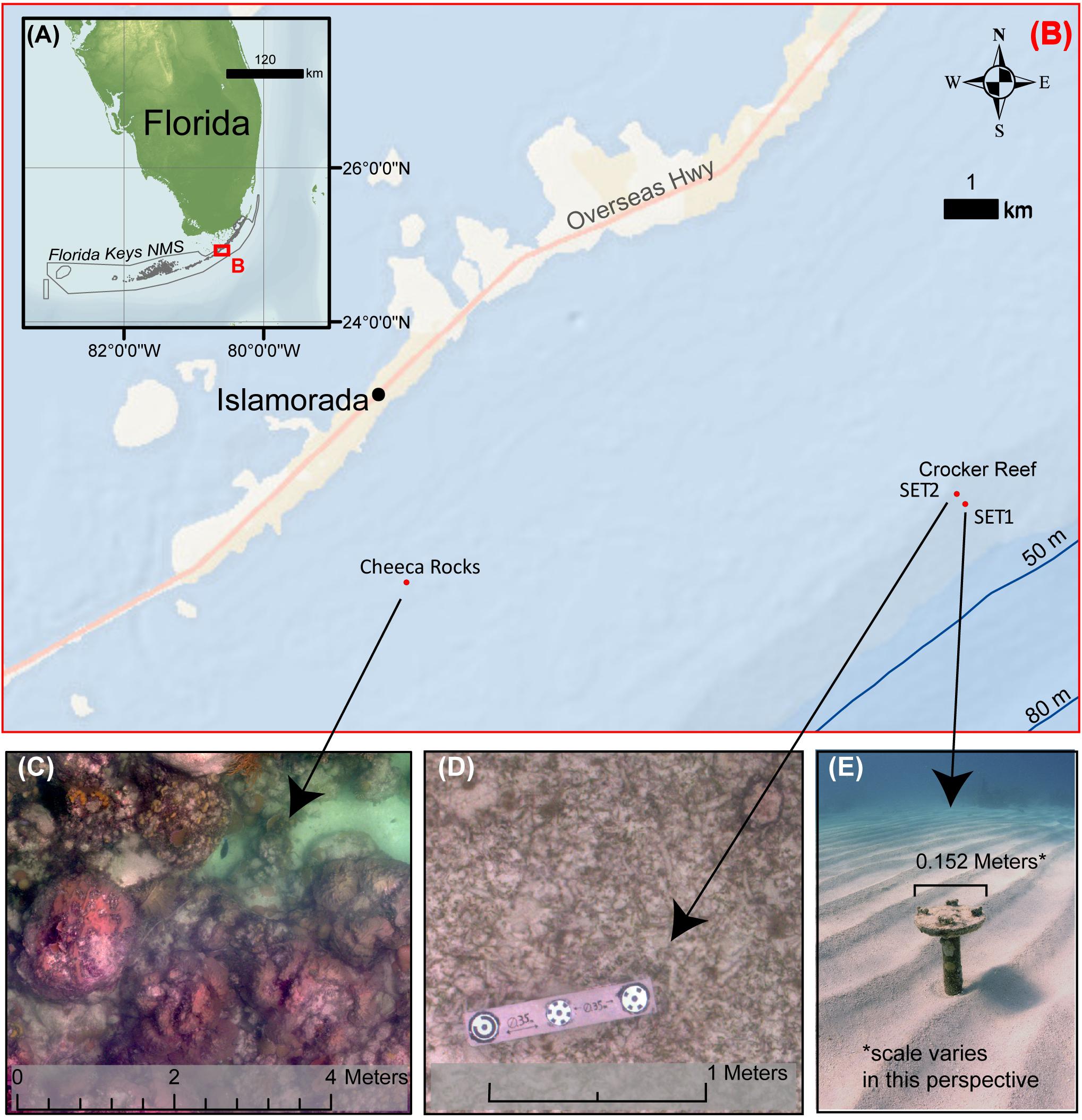
Figure 1. (A) Geographic location of fieldwork in the U.S. Florida Keys, global bathymetry (GEBCO), with operation area outlined. (B) Larger scale map of field site showing the locations of Surface Elevation Table (SET) stations and the Cheeca Rocks reef site location. (C) Example of the Cheeca Rocks coral reef orthomosaic generated from imagery collected using SQUID-5 (depth ranges from ∼2.5 m to over 4.5 m). (D) Sample of orthomosaic generated above SET station 2 from SQUID-5 imagery with scalebar and circular encoded targets attached (water depth ∼ 3.6 m). (E) Perspective photo of SET station 1 with protective cover plate installed showing sandy seabed and ripples typical at the site.

Methods

Instrumentation

During development of our underwater photogrammetry device, which is termed the SfM Quantitative Underwater Imaging Device with Five Cameras (SQUID-5; Figures 2, 3), several physical design goals were established, including the ability to hand deploy from a small vessel, easy disassembly and reassembly for shipping, structural rigidity, acceptable towing behavior in sea conditions of 1.5 m or less non-breaking surface waves from moderate swell, and survey speeds of 1.5 m/s or slower. The SfM analysis we intended required the design to incorporate precise synchronization between image capture and associated geospatial location of the image measured by the onboard GNSS. Additionally, early prototype testing on land suggested that a design with three or more cameras could both function in continuous mapping mode and allow for the generation of a complete 3D scene at every collection instance if the cameras were synchronized, fixed equidistant from each other at a spacing approximately 25% of their distance to the target surface, and oriented toward a central target point for maximum imagery overlap. Here we focus on the continuous mapping mode; the latter topic (scenes at each instance) will be addressed in future work. That noted, continuous mapping from multiple instances of three or more synchronized cameras appears to be advantageous because moving features – such as sand ripples, algae, fish, and debris – are collected at the same instant, which improves the reconstruction of these objects and reduces noise. A minimum of three overlapping images from slightly different perspectives is generally required to generate a 3D surface with SfM (Ullman, 1979). We built SQUID-5 conservatively by incorporating five cameras, each at different locations and view angles, to account for the fact that some imagery would likely be unusable. We correctly anticipated that a small camera vehicle towed on the open ocean surface would occasionally be oriented at an extreme angle relative to the seafloor due to surface wave action causing imagery from one or more cameras to be too oblique, and that the system would occasionally pass over debris or bubbles floating just below the surface, temporarily obscuring one or more camera views. The SQUID-5 design is summarized below, and further details including the system diagram and details of equipment and components can be found in the System Engineering Supplementary Material.

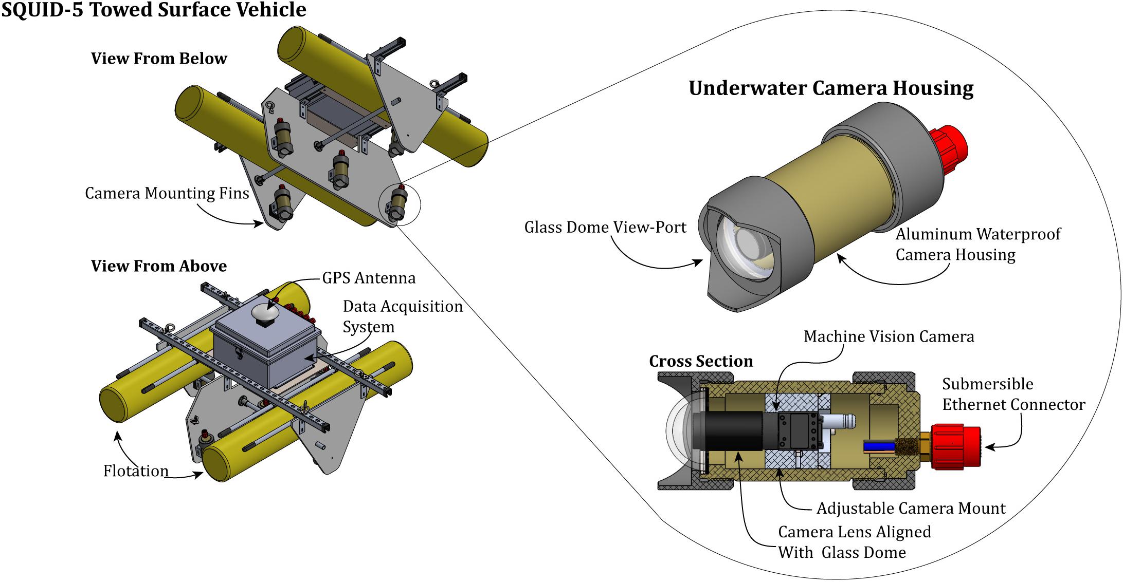
Figure 2. Diagram of the SQUID-5 towed surface vehicle and the waterproof camera housings with labeled components. The camera mounting mechanism aligns the camera axially with the dome and allows the camera to be adjusted fore and aft to accommodate various lens types and enable alignment with the glass port radius of curvature for minimal distortion.

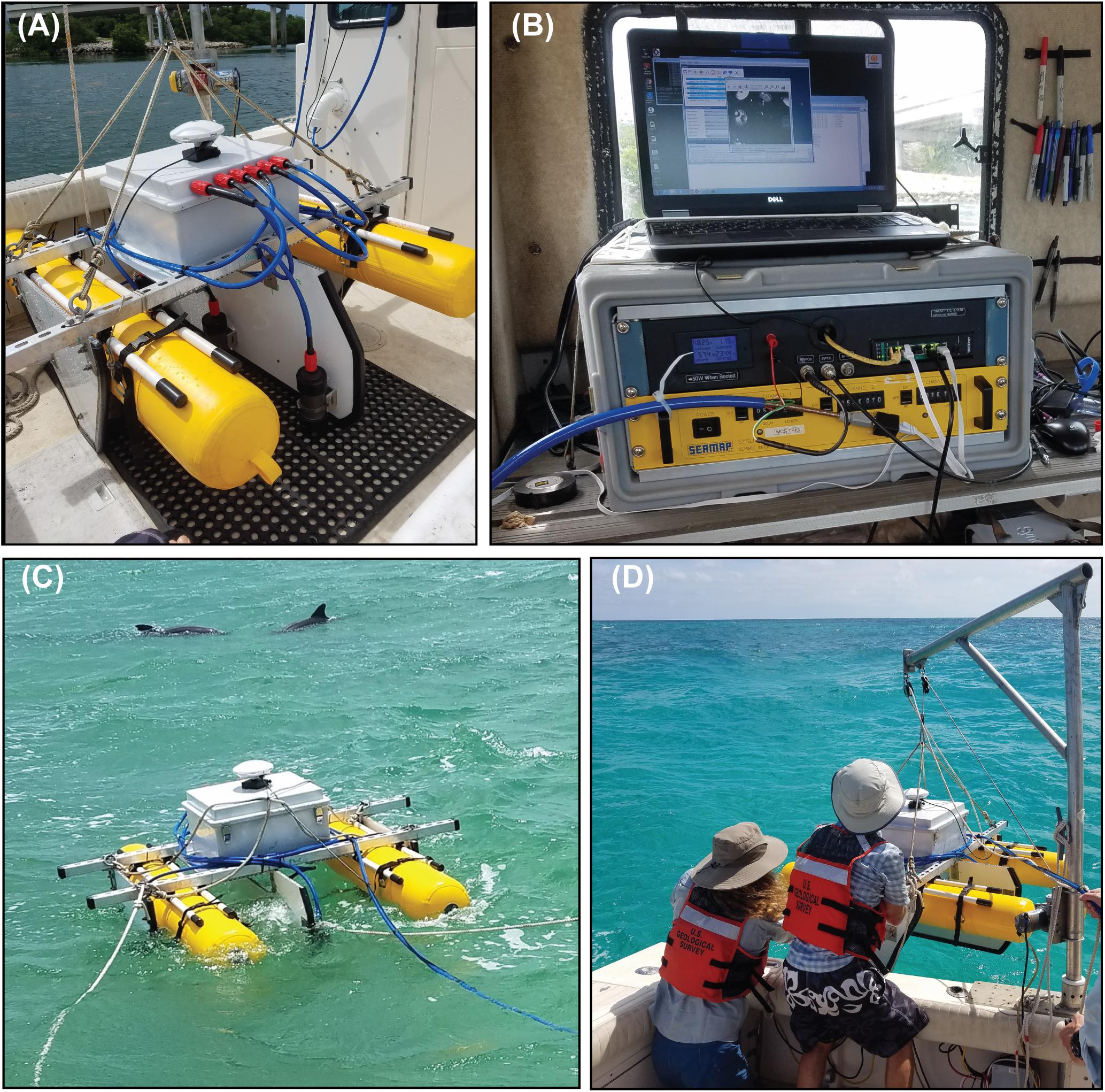
Figure 3. Photographs of field operations with the SQUID-5 towed surface vehicle: (A) the vehicle on the deck of the support vessel rigged for deployment; (B) the control station onboard the support vessel consisting of laptop, power supply, NTP time server, Ethernet hub, power supply, and trigger signal generating electronics; (C) the towed surface vehicle in operation; and (D) launch and recovery of the SQUID-5.

SQUID-5 Towed Surface Vehicle

We built SQUID-5 with a central downward-looking camera and four cameras orthogonally spaced roughly 0.5 m from the central camera (Figure 2). The camera orientation can be easily adjusted, and two setups were used during our operations. On the first deployment of the first day in the Crocker Reef area, we tested a setup intended to be used for efficient area mapping by creating a large across-track image footprint on the seabed, orienting port and starboard cameras 10° outward from the center camera’s field of view (FOV). This geometry still maintains approximately 100% overlap between the forward, center, and trailing cameras, and approximately 30% across track image overlap between the port, center and starboard cameras in 3.0 m of water. For the remainder of the fieldwork we maintained a camera orientation with all cameras pointed inward toward the center camera’s FOV resulting in nearly 100% overlap between all five cameras in 3.0 m of water.

The overall dimensions and weight of SQUID-5 enable it to be hand-carried, deployed, and retrieved by two people (System Engineering Supplementary Material). Structural support is provided by widely available aluminum strut channels and aluminum honeycomb panels, which combine to minimize flexure under loading. A fiberglass waterproof container is mounted atop SQUID-5 to contain the acquisition computer and provide a GNSS antenna mounting location (Figure 2). Buoyancy is created by two inflatable pontoons of urethane-coated canvas. The cameras are mounted to the lower portion of the honeycomb panels approximately 0.3 m below the water surface to minimize bubbles caused by towing turbulence (Figure 3). The mass of the aluminum camera housings mounted well below the vehicle’s center of buoyancy creates a stable arrangement for towing in seas with wave heights up to 1.5 m.

Cameras and Housings

Performance criteria for the SQUID-5 required cameras and lenses with high quality optics and a reliable high-quality image sensor with stable performance, small size, and reasonable cost. We selected 5.0 MP (2448 × 2048 pixels) FLIR Systems Blackfly S Gigabit Ethernet (GigE) machine vision cameras, which have a global shutter, 3.45 μm sensor pixel size, 24-bit color, and up to seven frames-per-second capture speeds. Additionally, the small size and symmetry of these cameras (approximately a 30 mm cube) simplified the design and fabrication of waterproof housings (Figure 2). Several lens options existed for these cameras, and we chose the Fujinon HF6XA-5M 6 mm fixed focal length lens, which has a 74.7° horizontal FOV and a 58.1° vertical FOV. At a design target of 3.0 m above the seafloor, an image from this camera and lens captured 4.57 m horizontally (across-track) and 3.34 m vertically (along-track), with a ground sample distance (GSD) of ∼1.725 mm at nadir (Matthews, 2008; Newman, 2008). Since the camera housings were built using glass dome viewports (see below), these GSD estimates were not significantly affected by water refraction of light. During data collection, the focus and aperture settings were fixed, while camera gain and shutter speed were adjusted as needed for each collection area using custom camera control software developed for this project.

Custom underwater camera housings were designed and built for SQUID-5 to minimize optical distortions and accommodate a range of lens options (Figure 2). Hemispheric BK7 glass domes were used for the camera viewport to minimize variations in focal length, FOV, radial and chromatic distortion, all of which are known limitations of flat ports in underwater photogrammetry (Nocerino et al., 2016). In addition, the hemispherical dome enabled the option of a more wide-angle lens if needed and increased the focus depth-of-field by approximately 33% for the same aperture setting over the flat port alternative (Menna et al., 2016). Cameras were mounted in the housings such that the camera lens nodal point was aligned with the center of the dome radius. With our chosen aperture of f5.6, the underwater focus depth-of-field was approximately 1 m to ∞.

GNSS and Camera Positioning

Positions of the cameras during each image capture instance were referenced to survey-grade GNSS measurements from a Trimble R7 GNSS receiver with a Trimble Zephyr-2 GNSS antenna mounted atop the SQUID-5 towed surface vehicle (Figure 2). Raw GNSS data were processed against base station data from a continuously operating reference station (CORS) in the Florida Permanent Reference Network (FPRN). The CORS station used (FLPK) was within 10 km of all survey sites and provided 1-hertz dual-frequency GPS and GLONASS data. The raw base and rover data were combined with precision ephemeris data and post-processed in Novatel’s Grafnav (v. 8.80) software suite, resulting in trajectories with RMS errors of 1.7 cm horizontal and 3.8 cm vertical. Timestamps from each trigger event were then imported into Grafnav and the interpolated antenna positions exported. All data are referenced to the NAD83 (2011) coordinate system and exported as both geographic and projected (UTM Zone 17N) coordinates, with both ellipsoid and orthometric (NAVD88 GEOID 12B) heights.

The existing CORS network was used for Post Processed Kinematic (PPK) GNSS position refinement out of convenience but it was not required. A similar level of accuracy is possible without the existence of the CORS network (or any other) by installing a temporary GNSS base station 24 h prior to the mapping fieldwork to refine its locally measured location. Once the base location is established it can then be used to record data continuously and simultaneously during the mapping fieldwork for later use in refinement of the mobile GNSS’s position data through post processing. The error of the mobile GNSS PPK locations are a function of distance from the base station, therefore the baseline distance should be minimized. Although the single baseline distance can acceptable to a distance of 30 km (Allahyari et al., 2018).

To translate the single PPK GNSS antenna position to individual camera locations, offset distances from the nodal point of each camera to the GNSS antenna phase center were measured using SfM. This included photographing SQUID-5 in the laboratory with machined scale bars temporarily mounted on the vehicle. Seventy-four photos from multiple angles were used to develop a SfM point cloud with point spacing less than 1 mm. Distance measurements from the cameras to the GNSS antenna were calculated in each camera sensor frame of reference using CloudCompare (version 2.10.2) and were included as initial estimates of the GNSS lever arm distances in the SfM analyses.

System Synchronization

To ensure images were collected at the same instant that GNSS location events were recorded, we used an electronic signal generator which triggered each system simultaneously through a shared voltage pulse (10-volt square wave) from the support vessel (see details in System Engineering Supplementary Material). Manufacturer’s specifications suggested that signal propagation delays should be less than 50 μs for the cameras and less than 1 μs for the GNSS. Therefore, maximum uncertainty in the relative position caused by timing errors during image capture was approximately 0.08 mm at a maximum survey speed of 3.0 knots (∼1.5 m/s), which is well below the PPK GNSS horizontal uncertainty of approximately 1.7 cm and was therefore considered negligible.

Data Acquisition

The acquisition computer was located directly on the tow vehicle in a waterproof housing (Figure 2). It was remotely controlled with a second computer located on the support vessel using Microsoft’s Remote Desktop application over a wired network connection (Figure 3). Both the control and acquisition computer system clock times were maintained using a GPS-based network time protocol (NTP) server located on the support vessel. To facilitate a rapid rate of data collection, four 2 TB solid-state hard drives were installed in the acquisition computer and configured as a high speed striped (RAID 0) array for a total storage capacity of approximately 8 TB and a sustainable write speed of over 300 MB per second. Each camera was connected directly to the data acquisition computer via its own dedicated GigE port.

Study Site

The Florida Keys Reef Tract parallels the 240-km-long Florida Keys island chain and extends from southeast of Miami to the Dry Tortugas in the Gulf of Mexico (Lidz et al., 2008). This barrier reef is approximately 6–7 km wide and numerous patch reefs are located in a shallow lagoon at water depths of approximately 3–6 m. The Florida Keys have a microtidal environment with tides less than 1 m. Field operations were conducted at Crocker Reef and Cheeca Rocks, both within the Florida Keys National Marine Sanctuary. These sites were chosen for their diversity of benthic settings, ease of access from a small boat, and history of scientific investigations, including previously installed Surface Elevation Table (SET) stations (Figure 1). Crocker Reef is a barrier reef located approximately 11 km east of the town of Islamorada, Florida, and is primarily a senile reef characterized by eroding coral reef topography, extensive bare sand, coral rubble, and seagrass habitat with average water depths less than 10 m. Two pre-installed SET stations were located at the Crocker Reef sites (Figures 1D,E). Cheeca Rocks is a small patch reef located approximately 2.5 km southeast of Islamorada, Florida, within a Sanctuary Preservation Area of the Florida Keys National Marine Sanctuary with complex topography. No pre-installed ground controls were located at Cheeca Rocks. Water depths at this study site were approximately 2–5 m as measured by the support vessel’s echo sounder.

The SET stations were installed at the site in August of 2014 by the USGS Coastal and Marine Science Center of St. Petersburg, FL, United States, for the purpose of tracking relative change in the seafloor bed elevation over time using a portable leveling device (Lynch et al., 2015). To ensure stability, the SET stations were fixed in place by drilling vertically to the depth of the Pleistocene layer, driving an aluminum rod into the hole until firm resistance, trimming the rod to length, attaching and leveling the SET station cap, and cementing the rod in place. Once installed, the locations of the SET stations were measured with a survey-grade GNSS by temporarily erecting a tripod directly above the station using a bubble level and weighted line to align and center a GNSS antenna mast over the center of the SET station caps. For maximum possible accuracy, the antenna locations were further refined in post-processing to correct for local atmospheric effects using data simultaneously collected with a nearby land-based stationary GNSS. Finally, antenna positions were translated to the SET station cap positions by applying offsets measured while the tripod was in place (Table 1). The uncertainties of these measurements were approximately 6 cm horizontally and 4 cm vertically, owing to the imprecision of the leveling devices and the accuracy of the GNSS measurements (Table 1).

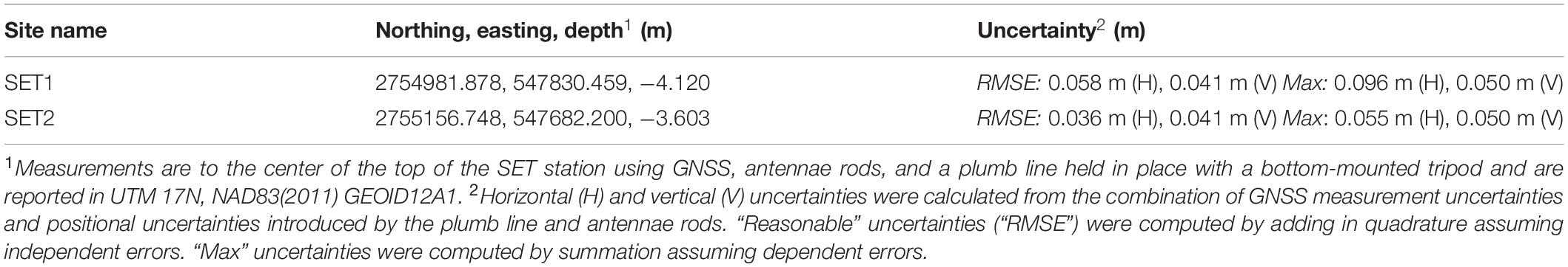
Table 1. Coordinates of the Crocker Reef Surface Elevation Table (SET) stations as measured by a survey-grade Global Navigation Satellite System (GNSS).

It is important to recognize that the significance of the pre-installed SET stations with known geo-spatial coordinates located within the study site was only that they provided a means to measure the geo-spatial accuracy of seafloor data products generated using data from SQUID-5 and SfM. The SET station locations were not used as ground control during SfM processing. Geo-spatial SET station locations were measured independently using the newly generated SQUID-5 bathymetric data products and then compared to the previously GNSS surveyed coordinates from 2014. This is described further in the section “Accuracy Assessments of SfM Products”.

Field Operations

Seafloor imagery and associated geo-locations were collected with SQUID-5 during small boat operations based out of Islamorada, Florida, on July 11–13, 2019 (Figure 1). The USGS R/V Sallenger (8-m long Parker 2530 with enclosed cabin) was used as the host vessel with real-time acquisition and monitoring set up inside the cabin (Figure 3B). A second team of USGS science personnel used another small boat, the USGS R/V Halimeda (8-m long, modified Oceans Formula with an open deck), to attach circular encoded targets to SET stations and deploy a three-dimensional scale bar, both of which were used for data validation (Figure 4).

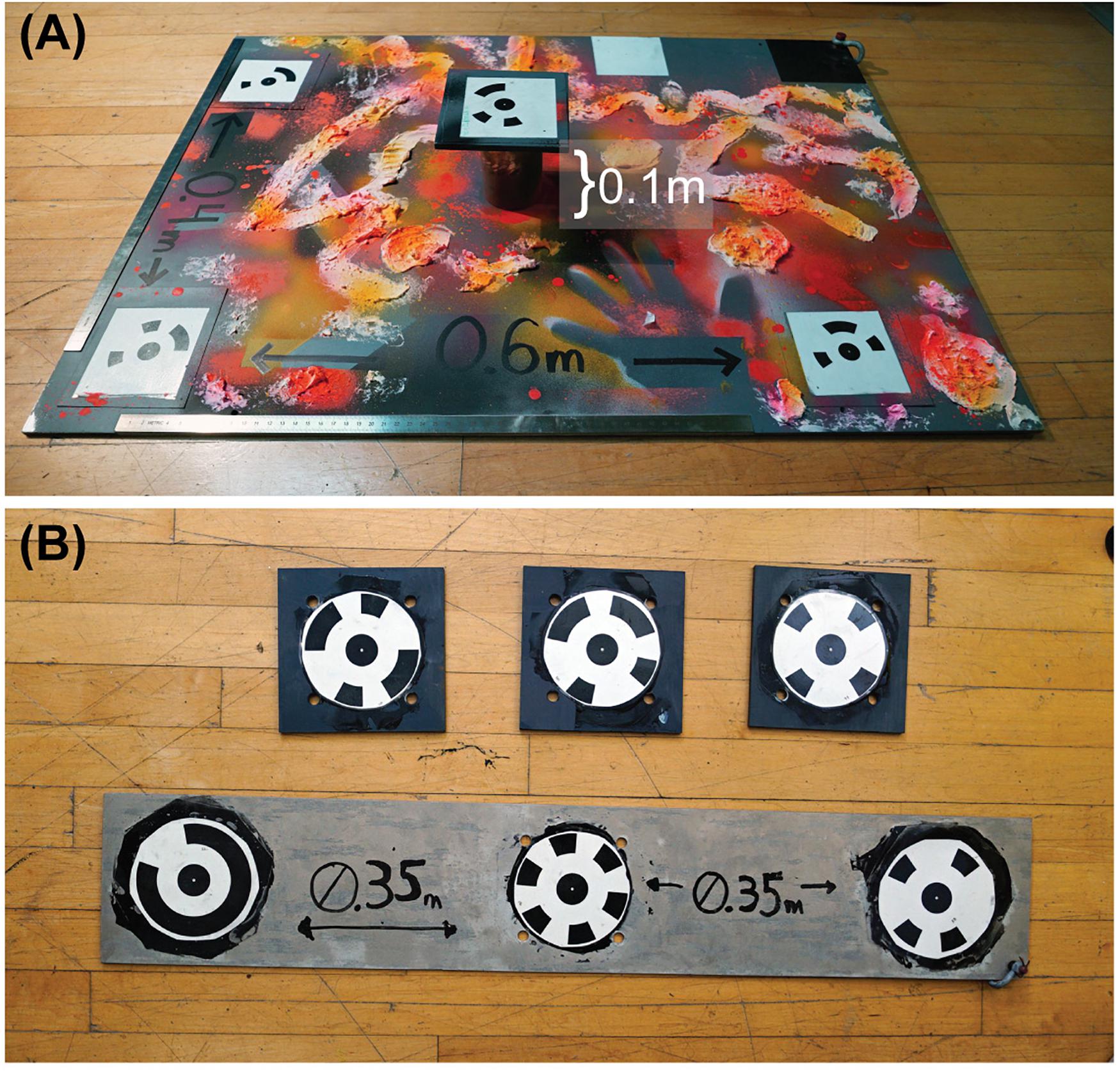
Figure 4. Machined scale bars and targets for accuracy assessment during field operations: (A) submersible camera calibration plate including precisely positioned circular encoded targets in three dimensions, painted with texture to assist Structure-from-Motion (SfM) photogrammetry reconstruction of the plate and with black and white squares for exposure and color balance adjustment; (B) individual circular encoded targets and a linear scale bar for mounting precisely to the Surface Elevation Table (SET) stations.

The primary purpose of the field experiment was to evaluate SQUID-5’s capabilities and limitations. Therefore, our focus at the two SET stations was to acquire data in order to assess data accuracy, precision, and reproducibility. The Cheeca Rocks site was selected to evaluate system performance and its ability to resolve complex benthic features over a high relief area (Figure 1C). Data from several adjacent passes at all three locations were combined to create seamless maps of several hundred square meters, demonstrating the potential for mapping larger areas of contiguous reef at both sites (Figures 5–8). Notably, SQUID-5 is a tool intended to map relatively small areas but at very high resolution when compared with more traditional mapping technologies such as sonar or airborne lidar. For example, mapping a 100 m × 200 m area of seafloor in 3 m of water depth would require an estimated 2.5 h of boat operations. This estimate assumes only 50% efficiency during collection in order to allow for vessel turns and the difficulty of navigating a vessel along tightly spaced survey lines.

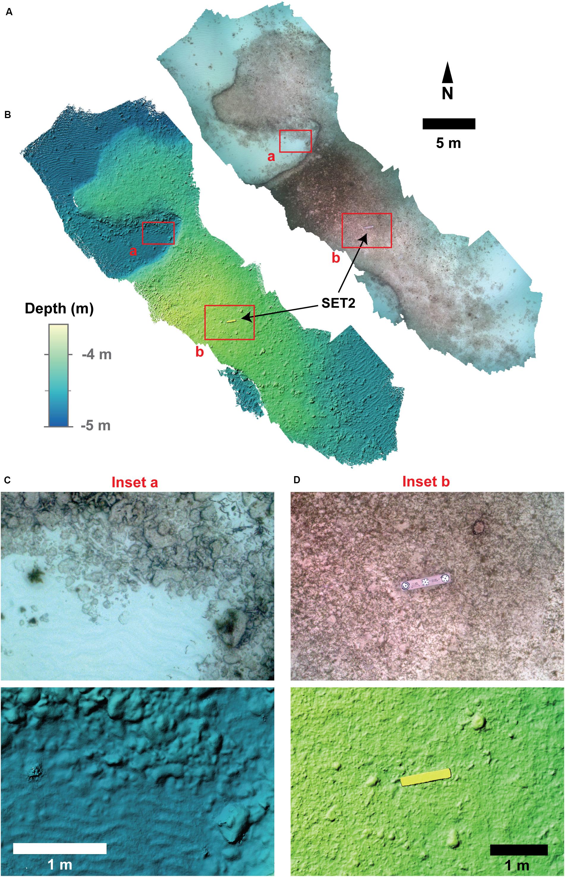
Figure 5. (A,B) Mapped orthomosaic and bathymetry obtained from three survey passes of the Surface Elevation Table (SET) station 2 site with the SQUID-5 system. The shaded relief bathymetry is shown for a digital surface model (DSM) derived from the Structure-from-Motion (SfM) dense point cloud. The spatial resolution of the photo mosaic and DSM are 2.1 mm and 4.1 mm, respectively. (C,D) Highlights of the benthic maps of the site, including sand, rubble, eelgrass and the scale bar mounted on the SET station 2 monument.

To achieve optimal SfM results, our image collection rate was selected such that sequential images had at least 60% overlap and angular change between features in sequential images would not exceed 15° (Matthews, 2008). As detailed in the Optimal Image Spacing Supplementary Material, the limiting factor for our wide-angle lens selection was the 15° angular change maximum, and, considering a target distance of 3 m, we calculated that a 2 Hz collection rate at a maximum survey speed of 3.0 knots (∼1.5 m/s) would adequately meet this requirement. Actual operating conditions commonly included survey speeds of 1.5–2 knots (∼0.8–1 m/s) and imagery collection at 2 Hz (Table 2). However, the vehicle was occasionally allowed to drift slowly over features of interest to evaluate the effects of greater photo densities. Over the course of fieldwork, sea state ranged from calm to over 1 m wind chop. Water clarity at both SET stations was such that the seabed was clearly visible in all the imagery. Turbid conditions at Cheeca Rocks made it difficult to clearly discern the seafloor in many images collected in water depths greater than approximately 4 m. Ambient lighting ranged between partly cloudy and overcast, which limited the effects of light ray caustics that can inhibit photogrammetric reconstructions (Agrafiotis et al., 2018).

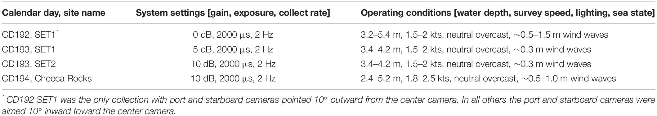
Table 2. Environmental conditions and system settings used at each survey site.

SfM Analyses

The SfM processing was done with Agisoft Metashape software (version 1.5.2, build 8432) using general single-collection techniques. The SfM analyses were performed in a manner to maximize seabed returns and limit errors from insufficient or excessive photo coverage. Higher photo densities from drifting at slow speeds resulted in overly noisy SfM point clouds, largely from the small separation distances between photos with respect to water depth. To minimize these errors, the complete photo sets of each study area were subsampled such that minimum GNSS measured spacings between independent collection instances were at least 0.75 m (see Optimal Image Spacing Supplementary Material). This data reduction step dramatically reduced the noise in the final SfM products.

For each survey site, the subsampled photo quintets were combined with GNSS positions and camera-to-GNSS-antennae distance vectors (lever arm offsets) and aligned with independent lens models derived for each camera using camera-specific image subsets within Metashape. The computed camera positions and lens models were then refined using three statistical tools (reconstruction uncertainty, projection accuracy, and reprojection error) in Metashape to eliminate poorly constructed tie points. With trial and error, we found that threshold values of 20, 8, and 0.4 (entered as unit less parameters) for these statistical tools, respectively, resulted in good alignment and adequately dense tie point distributions in both high-relief reef settings and relatively flat sandy areas.

Once the photo alignment and lens models were optimized, dense point clouds were generated with Metashape using high point density and moderate filtering settings. Dense point clouds were used to generate digital surface models (DSMs) and photo orthomosaics for each study site using the Metashape default cell spacing, which ranged between 3.8 and 4.1 mm for the DSMs and 2.0 and 2.2 mm for the orthomosaics. The DSM and orthomosaic products were generated primarily for visualization, whereas most of the analyses were based on the high-density point clouds. For the SET station 1 site, two independent surveys were conducted using different SQUID-5 camera orientations and on different dates to evaluate the reproducibility of the data at this site.

Accuracy Assessment

Accuracies of the resulting data were evaluated for both local-scale measurements (decimeter to meter) and georeferenced map products. Linear measurements in the SfM point clouds, which included both horizontal and vertical directions, were compared with precisely measured dimensions of scale bars placed in two study sites (Figures 1D, 4, 5D). Printed targets were physically attached to the scale bars at precise spacings with submillimeter accuracies. The targets were detected in imagery with algorithms available in Metashape or manually identified in photos where the detection algorithms did not select them, and then Metashape was used to calculate distances between targets.

Three-dimensional georeferenced point accuracies were evaluated by comparing SfM-derived positions and elevations of the two SET stations with their previously measured GNSS-surveyed positions and elevations acquired at their time of installation in 2014. At SET station 1, two independent SfM measurements were made with SQUID-5 using different camera set-ups and on separate days (Table 2). SET station 2 was mapped on a single survey day.

The reproducibility of the SfM bathymetric surfaces was assessed with two independent surveys of the SET station 1 site. An area of overlap, which was roughly 20 m by 10 m and included elevated sessile reef and sandy regions with pieces of reef rubble, was obtained in both surveys and analyzed for differences. The reef and rubble were assumed to be stationary between the two surveys, such that they were used in direct point cloud-to-point cloud comparisons. All cloud-to-cloud comparisons were made within CloudCompare using the Multiscale Model to Model Cloud Comparison (M3C2) algorithm, which computes total and directional differences normal to the local surface of one of the point clouds (Lague et al., 2013).

The results of the overlapping surveys were assessed both by using the uncorrected, or raw, SfM output of both surveys and by correcting offsets between the SfM point clouds using locations on hard features that were assumed to be fixed to remove biases. Three bias correction techniques were used: (i) three-dimensional translation of a point cloud by northing, easting and vertical constants derived from comparisons of a single, easily identified point on the ridged structure of the reef (“single-point bias correction”), (ii) three-dimensional translation and rotation of a point cloud using differences in three points easily identified on the reef and in the rubble area (“three-point bias correction”), and (iii) use of the positions of three points on the reef and rubble as SfM markers for a second reprocessing generating a complete reanalysis with the SfM technique (“three-point iterative SfM correction”).

Results

Benthic SfM Products

With SQUID-5 we collected photo quintets and associated GNSS positions that were used with SfM processing to generate point clouds, surface models, and orthomosaics (Warrick et al., 2020) of complex seafloor structure that included biotic and abiotic components of benthic habitat such as coral heads, rubble, and sandy ripples (Figures 5, 6, 8). To verify the capability for multi-pass seamless area mapping with SQUID-5, data from three survey passes of the SET station 2 site were processed simultaneously to generate nearly continuous point cloud, elevation, and photo mosaic products for an area approximately 500 m² (Figures 5A,B). Close examination of these data reveal that the SfM products characterized the 3D extension of reef, rubble, sand ripples, benthic organisms, and the scale bar placed atop the SET station 2 (Figures 5C,D).

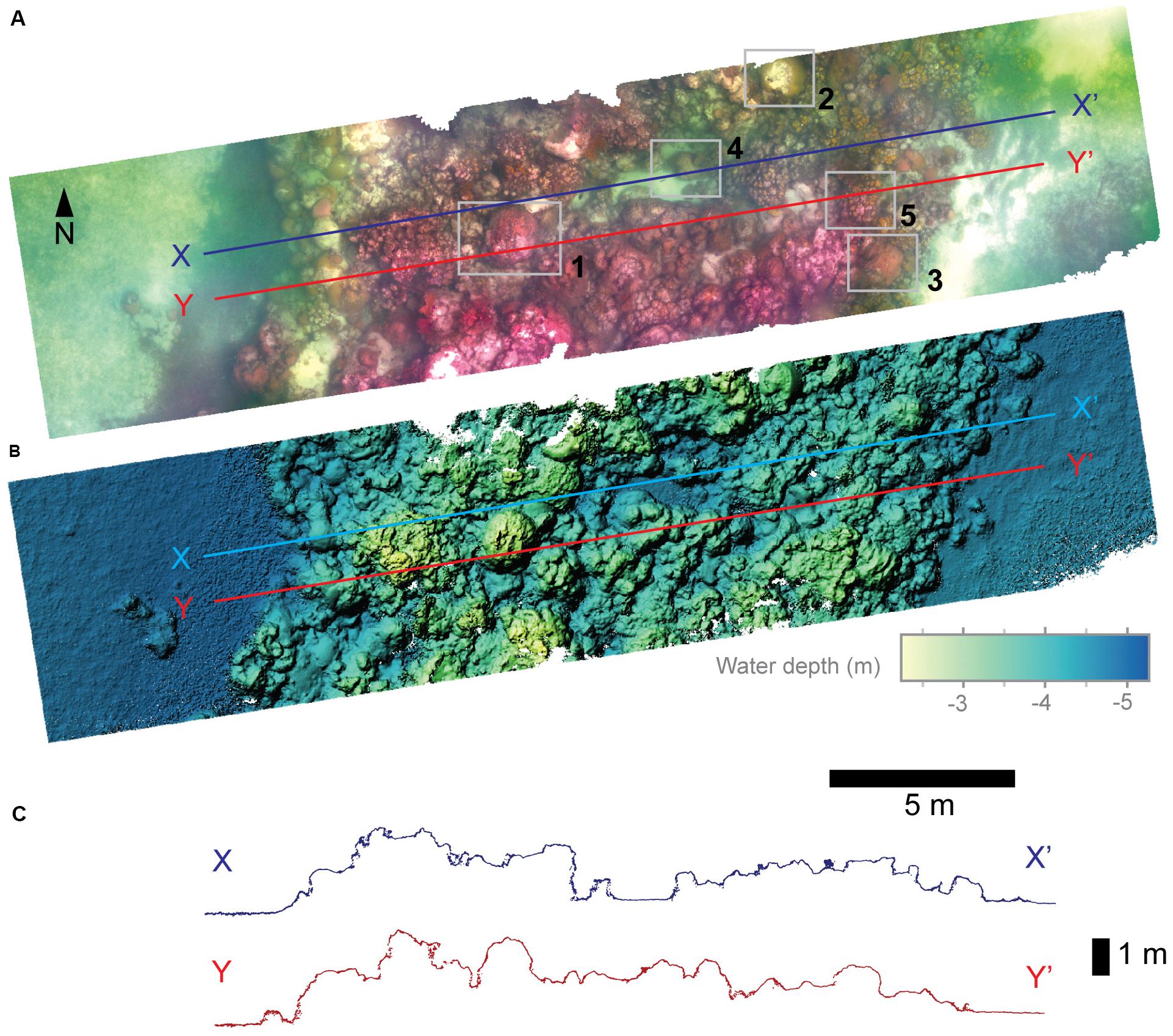
Figure 6. (A,B) Mapped photo mosaic and bathymetry obtained from two survey passes of the Cheeca Rocks site with the SQUID-5 system. The shaded relief bathymetry is shown for a digital surface model (DSM) derived from the Structure-from-Motion (SfM) dense point cloud. The spatial resolution of the photo mosaic and DSM are 2.2 and 3.8 mm, respectively. (C) Elevation profiles of the Cheeca Rocks reef derived from the SfM dense point cloud. Locator boxes (1–5) are detailed in Figure 7.

The ability of SQUID-5 to capture details of complex topography can be seen by examining profiles of SfM data collected at Cheeca Rocks, which includes live coral, sand flats, and vertical-to-overhanging slopes (Figure 6A inlay 1, 4, and 5). This site was mapped in detail using the 2.2 mm resolution photo mosaic and millimeter-scale point cloud (Figure 7). Profiles of the point clouds through these coral heads reveal detailed topographic information on the coral surfaces and can detect other centimeter or sub-meter scale benthic organisms such as gorgonians (Figure 7A.1). Vertical to overhanging sections of the coral heads were commonly less well resolved and more highly variable than the uppermost surfaces, indicating these areas are more challenging to map and illustrating a limitation of surface-towed cameras for SfM methods.

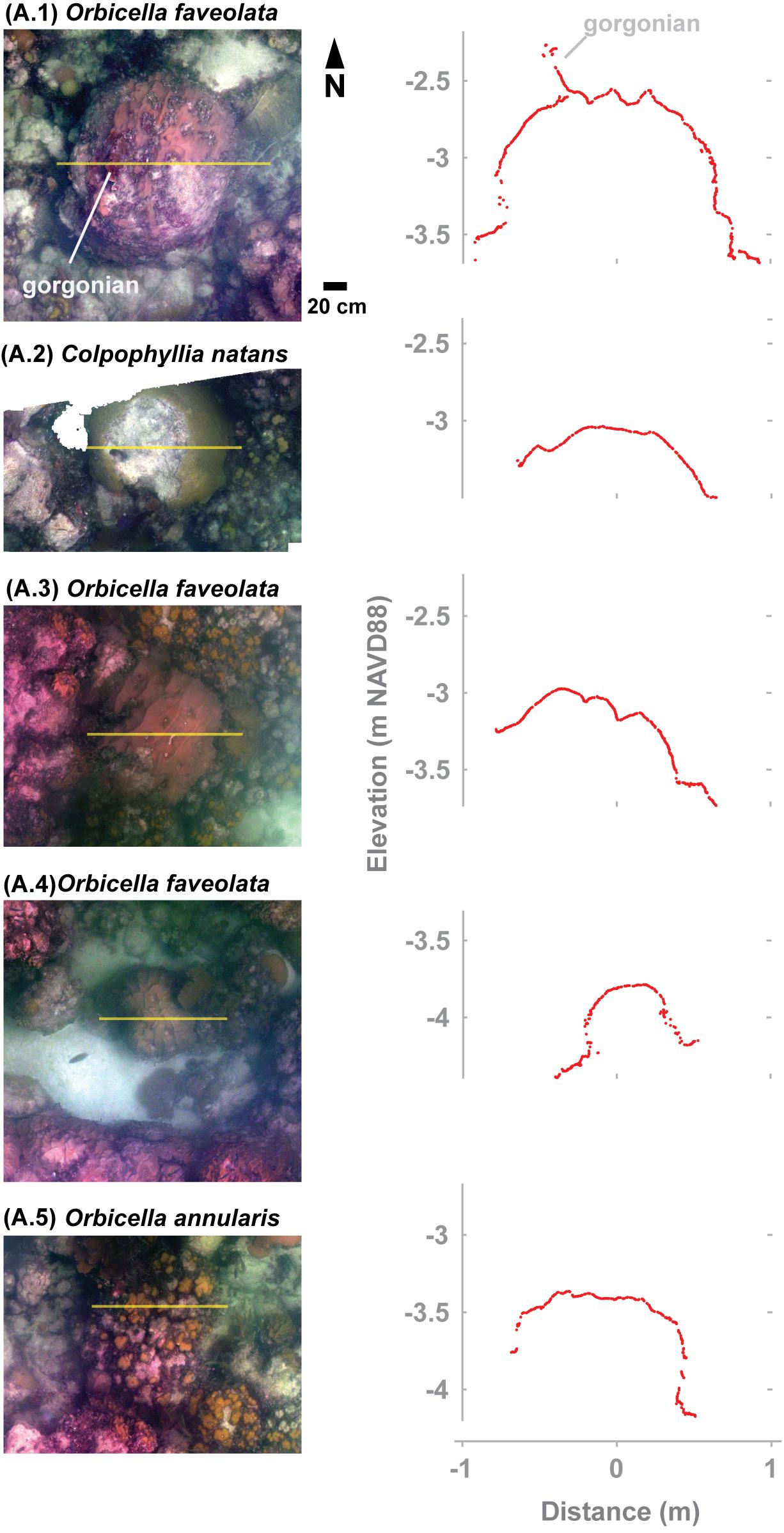
Figure 7. Photo mosaics and elevation profiles for several coral heads mapped at the Cheeca Rocks site and highlighted by locator boxes 1–5 shown in Figure 6A. Coral species include Mountainous Star Coral (Orbicella faveolata), Boulder Brain Coral (Colpophyllia natans), and Boulder Star Coral (Orbicella annularis). The profile in (A) includes a sea fan, or gorgonian (Gorgonia ventalina). Profiles were derived from the original Structure-from-Motion (SfM) point cloud using all points within ±1 mm of the profile transect.

Lastly, two independent multiple-pass surveys were conducted approximately 24 h apart on the SET station 1 site and revealed a broad sandy plain and a senile reef (Figure 8). We did not attempt to repeat the same survey lines on the 2 days, so the total area covered differed. However, substantial changes were observed in the area intersected by both surveys, most markedly in the orientation and complexity of the sand ripples, which were likely caused by time-dependent changes in ocean waves (Figure 8). For example, the orientation of the sand ripples rotated clockwise by 15–40° with the greatest amount of rotation occurring adjacent to the reef, and the wavelength and amplitude of the ripples decreased by approximately 25 and 40%, respectively. The ripples on the second day of surveying were disturbed slightly from dive crew operations, as noted by the diver bag, calibration plate, marker buoy anchor and associated drag marks, and the measurement arm attached to the SET station (Figure 8). Hard features, including bedrock and a portion of the reef, were mapped during both survey dates and showed little change, which suggests that they can be used to measure differences in the SfM point clouds as detailed below.

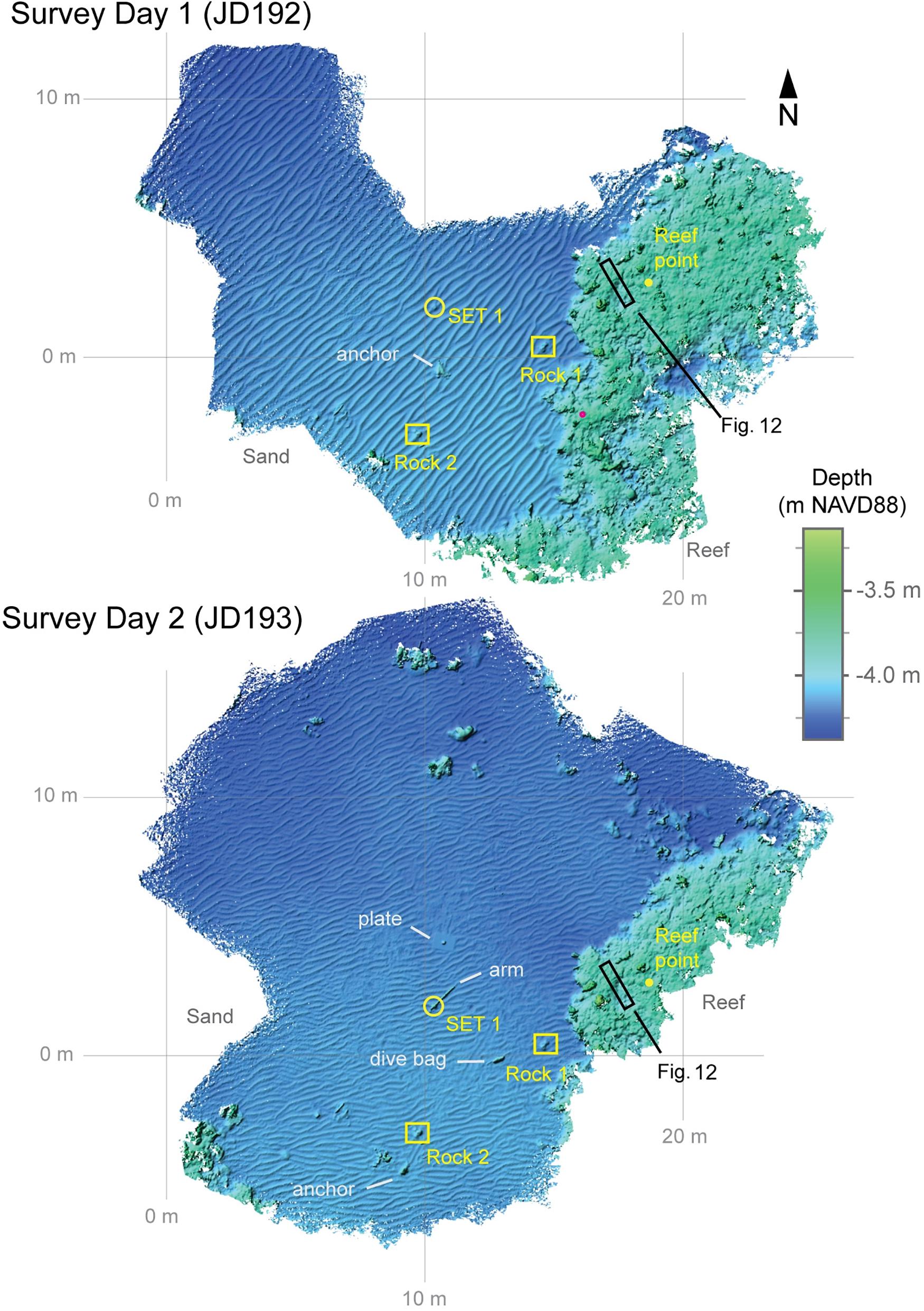
Figure 8. Mapped bathymetry obtained from several survey passes of the Surface Elevation Table (SET) station 1 site with the SQUID-5 system. Survey data from 2 days were collected and processed independently with our Structure-from-Motion (SfM) workflow. Shaded relief bathymetry is shown for the DSMs with spatial resolutions of 3.9 and 4.1 mm, respectively. The wavelength (approximately 0.3–0.5 m) and amplitude (approximately 0.02–0.04 m) of the sand ripples were similar between surveys; however, an approximately 40° change in orientation and complexity increase are readily observed. Locations of several features used for the analyses are labeled. Field crews were conducting SET measurements during the second survey day, as shown by the dive bag, anchor, and measurement tool arm on the SET site.

Accuracy Assessments of SfM Products

Measurements of the 3D scale bars generated with the SfM techniques differed from the actual values of the machined scale bars by less than 1 mm (scale length ranged from 10 cm to over 72 cm and the mean difference was 0.2 mm with a standard deviation of 0.5 mm; Table 3). Scaling by the water depth of each measurement, these errors ranged between 0.016 and 0.024% of water depth (Table 3). Thus, the SQUID-5 reliably produced sub-millimeter measurement accuracy both vertically and horizontally over distances of 10 s of centimeters on the seafloor.

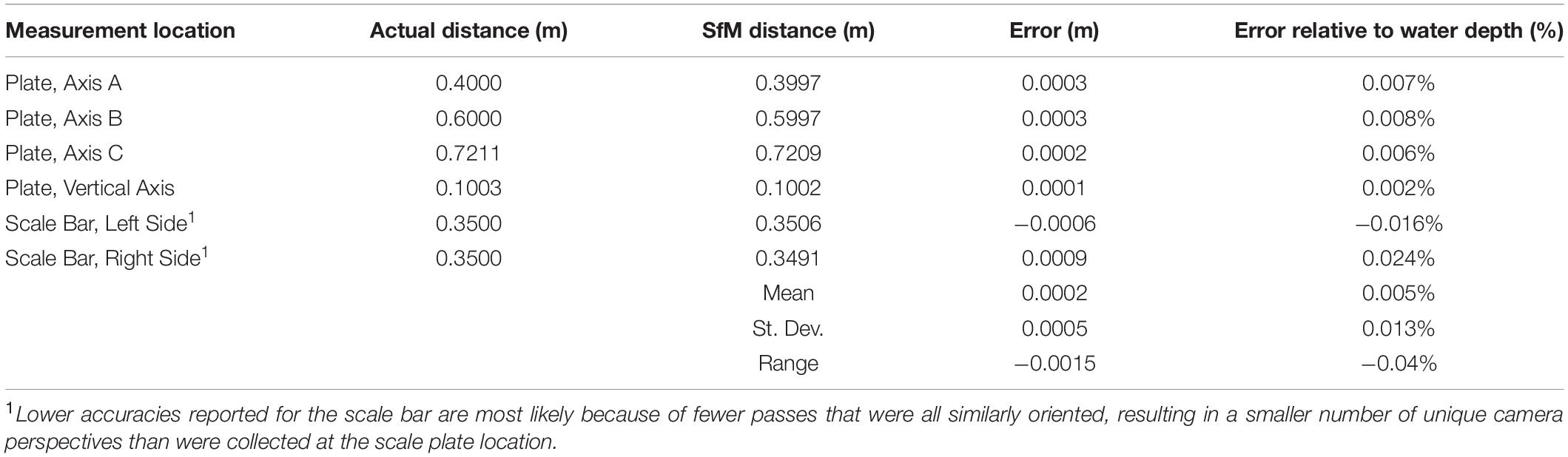
Table 3. Comparisons of SfM distance measurements using no ground control with machined scales placed on the seafloor.

The SfM-based position estimates of the SET station geo-spatial locations were within approximately 3 cm of the total uncertainty of coordinates previously acquired using GNSS surveys (Figure 9). As described in Section “Study Site,” prior SET station location measurements were collected using a survey GNSS attached to a tripod that was temporarily erected on the seafloor and extended above the water surface directly above the SET stations. Positional differences between the two measurements were greater in the horizontal directions than the vertical, which reflects greater error in the horizontal positions of the original GNSS surveys, owing to the difficulty of precisely leveling a tripod with a total height greater than 4 m in the open coastal ocean environment. The two independent measurements of the geo-spatial position of SET station 1 by our SfM methods produced results that differed by only 0.98 and 0.83 cm in the horizontal and vertical directions, respectively, which suggests that position reproducibility of this SET station was on the order of a centimeter (Figure 9A).

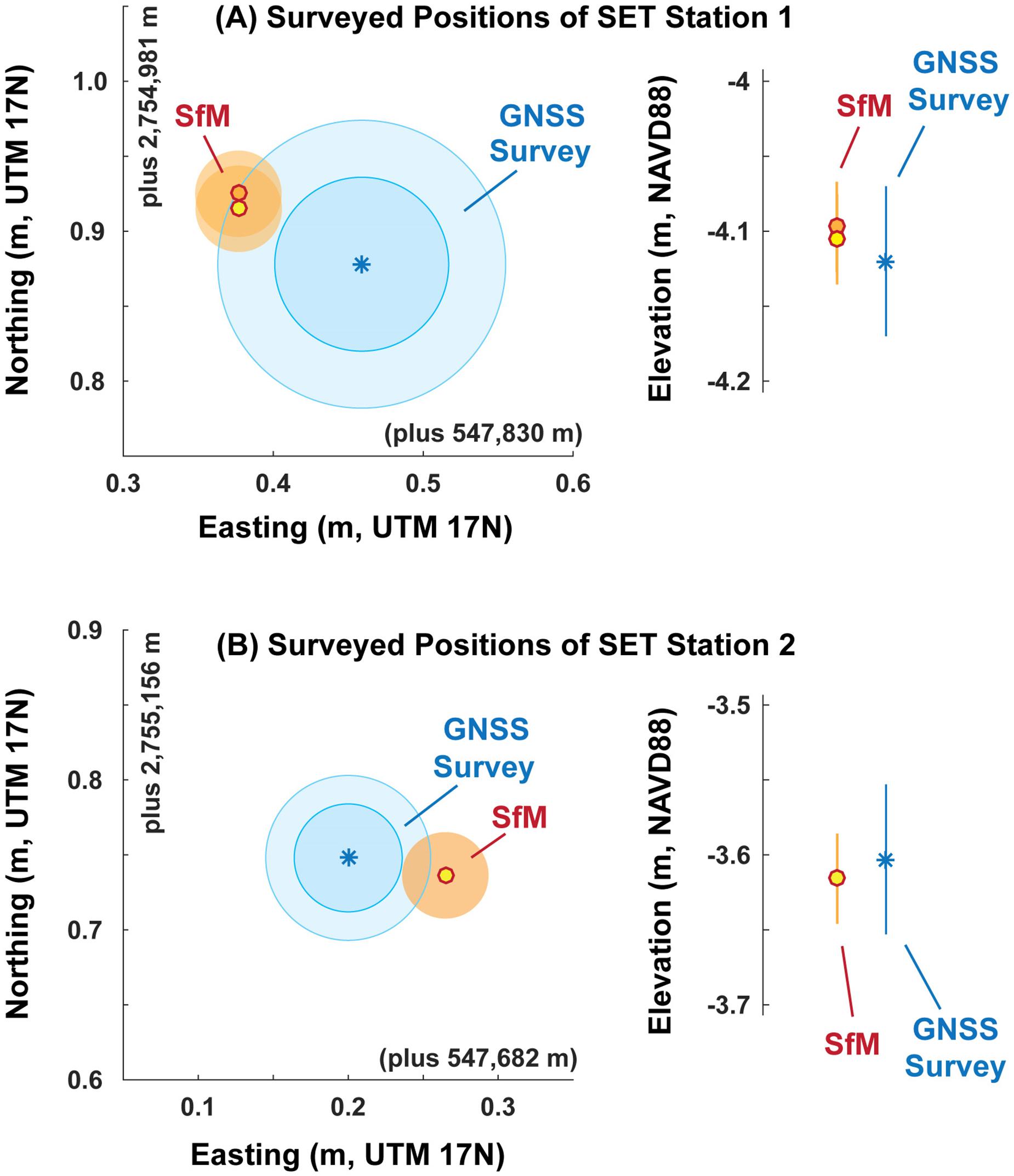
Figure 9. Comparison of the measured positions of the Surface Elevation Table (SET) stations 1 and 2 (shown in A,B respectively) from field-based Global Navigation Satellite System (GNSS) and Structure-from-Motion (SfM) with the SQUID-5 system. Greater uncertainty exists for the GNSS measurements owing to the leveling techniques during scuba conditions, and both “reasonable” and “max” uncertainties are shown for the GNSS measurements (see Table 1). Uncertainty of the SfM measurements assumed to be 3 cm, which is equivalent to the approximate uncertainty of the survey-grade GNSS measurement.

A more thorough analysis of reproducibility was conducted by comparing three areas of hard substrate at the SET station 1 site: two rocks in the sand and the overlapping portion of the reef contained in both data sets (Figure 10). Comparing the raw SfM output from the two independent surveys reveals that the sandy areas had complex changes associated with the reorganization of the ripples, but that the reef area had more spatially consistent offsets of roughly 1–4 cm, which increased toward the northwest (Figure 10A). These offsets were reduced markedly with the three bias correction techniques, approaching values less than 1 cm (Figures 10B–D). The single-point bias correction continued to have a positive slope in the computed offset (Figure 10B), whereas the three-point correction techniques had limited slope in the offsets (Figures 10C,D).

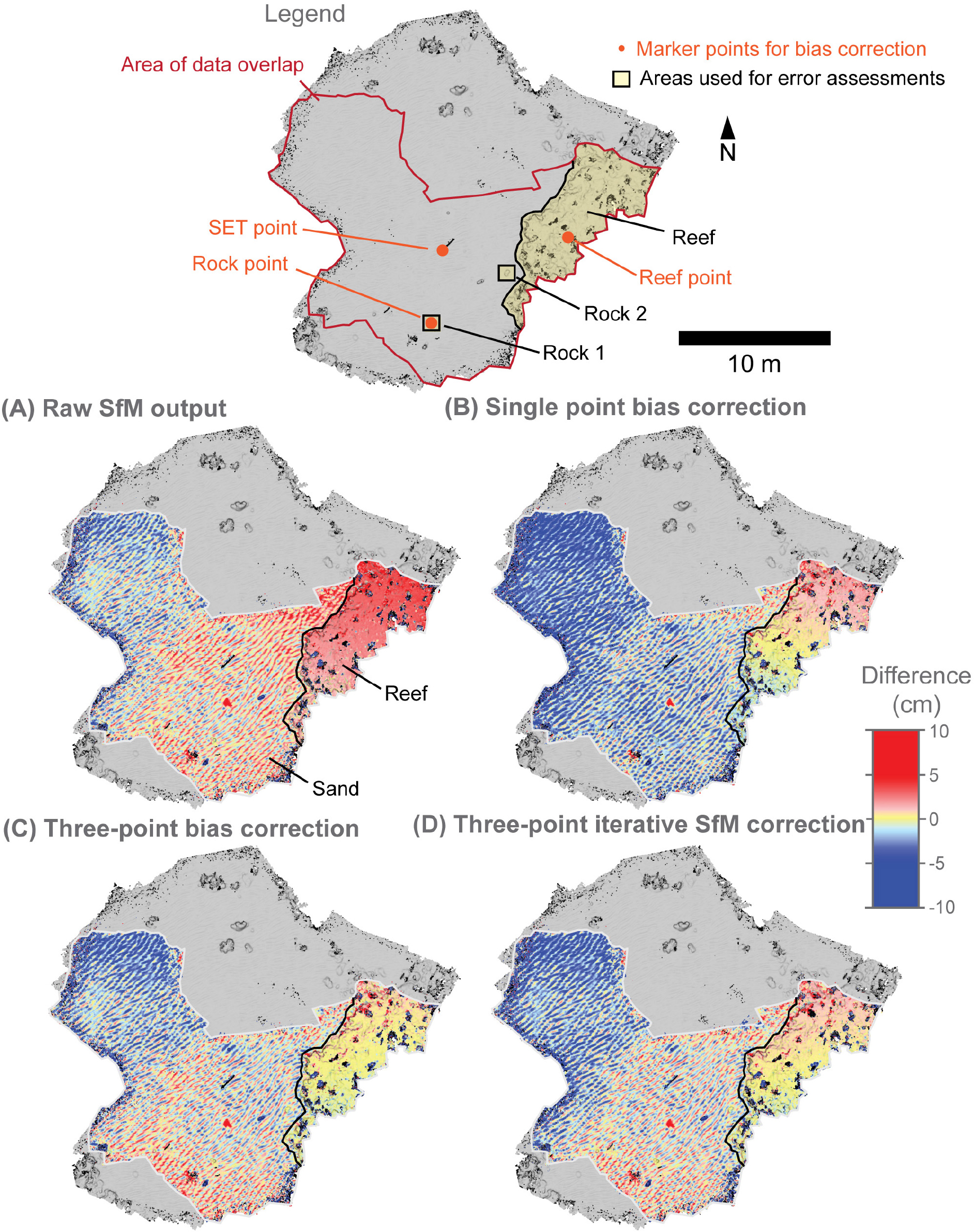
Figure 10. Difference measurements of the Surface Elevation Table (SET) station 1 site point clouds using the M3C2 measurement tool to test for reproducibility. The legend shows the area of data overlap for the surveys, marker points used for bias correction, and the three areas used for error computations. (A–D) Difference maps for the four comparative techniques, including raw Structure-from-Motion (SfM) output, single-point bias correction, three-point bias correction, and three-point iterative SfM correction. In each map, the reef area is highlighted with a black line.

A summary of the effect of the bias correction techniques shows that corrections dramatically reduced offsets between the two SfM surveys (Figure 11). For the raw SfM output, the mean difference of the three stationary areas ranged between 4 and 19 mm, and the variance of these differences ranged between 7 and 15 mm (Figure 11). The single-point bias correction shifted the overall errors closer to zero and brought variance to 4–8 mm. The smallest differences were measured for the two three-point correction techniques, which resulted in mean errors that were consistently within 2 mm and variances that were 2–4 mm (Figure 11).

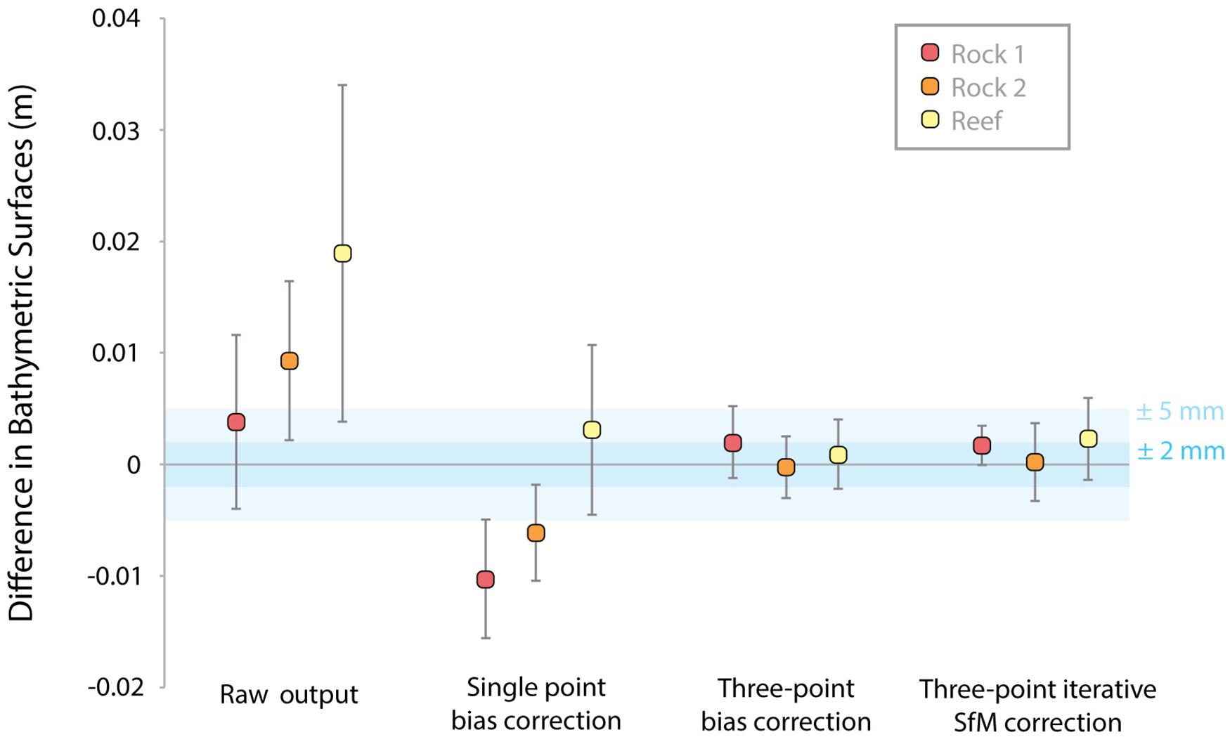
Figure 11. Summaries of the differences in stationary objects at the Surface Elevation Table (SET) station 1 site during the two surveys. Three different objects were used for measurements, the locations of which are shown in Figure 10, and four comparative techniques were used as detailed in the text. Differences computed from M3C2 measurements of the point clouds, and the mean and standard deviation of the measurements are shown with the point and error bars, respectively. Shading highlights differences that are ± 5 mm and ± 2 mm.

An example of the differences for the three-point bias correction technique is shown for a 2 m by 0.4 m transect of the SET station 1 reef that is complex and greater than 1 m away from the reef marker point (Figure 12). The shaded-relief bathymetries from the two surveys are quite similar, with an elevated region on the northern end that contains live coral and a depression near the southern end with some sand (Figures 12A–C). Differences in this bathymetry are generally low, with a mean and variance of 0.8 and 3.1 mm, respectively (Figures 12D,E). Differences in excess of several millimeters are apparent in a few locations, including an area with plausible actual change resulting from sand movement and two areas with overhangs that were reconstructed differently by the SfM algorithms but likely had no actual change (Figure 12D). This subset of the reef reveals that repeatability can be achieved with an uncertainty of a few millimeters for reef tops and flats, but that uncertainty increases in difficult to measure areas, such as overhangs.

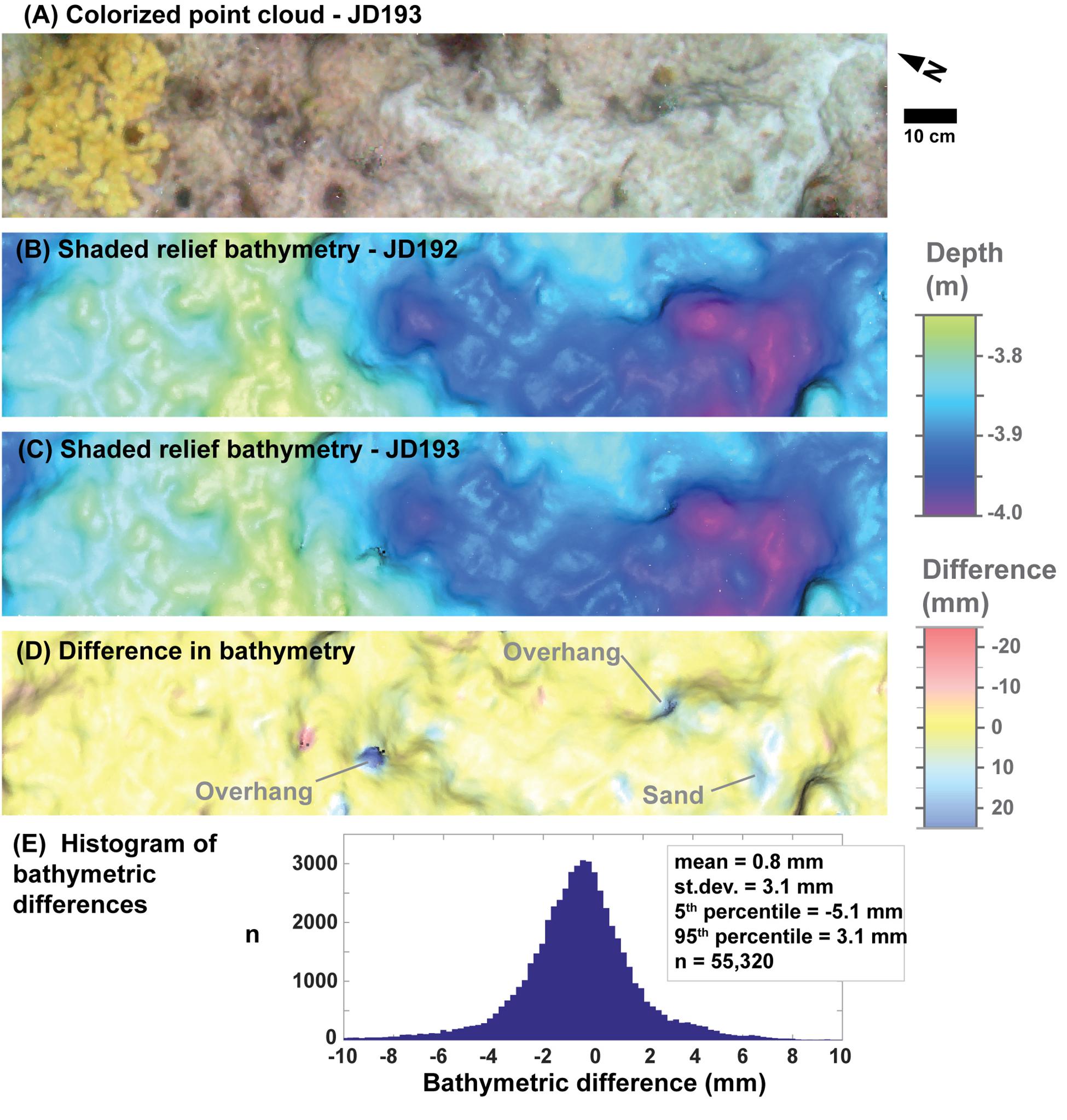
Figure 12. Survey-to-survey differences for a 2 m by 0.4 m section of the Surface Elevation Table (SET) station 1 site reef chosen for its spatial complexity and lack of bryozoans. Location of this inset is shown in Figure 8. (A) True color map of the point cloud showing live coral on the northern end of the transect and a depression with sand on the southern end. (B,C) Shaded relief of the bathymetric point clouds. (D) Difference between the two point clouds using the M3C2 measurement tool. Features with the greatest difference values are highlighted and described. (E) A histogram of the M3C2 difference measurements for this transect, including summary statistics of the distribution.

Discussion

A multi-camera SfM system was successfully developed and used for surveying benthic habitat of the Florida Keys, resulting in millimeter-scale resolution, ∼0.01% linear measurement uncertainty as a function of depth, and mm-to-cm scale positional accuracy, all without any independent, pre-existing ground control. Synchronization between the SfM cameras and the survey-grade GNSS allowed for detailed three-dimensional point clouds of reefs and surrounding areas that were confirmed to be accurate using linear scales, three-dimensional positions, and repeatability of mapped surfaces. Over live coral heads, the resulting SfM point clouds were dense and uniform except on steep or overhanging surfaces, where data densities dropped and became noisy (Figure 7). Combined, these capabilities will allow for highly accurate measurements of change on the tops and exposed sides of corals, rock outcrops, or other benthic structures, but less accurate measurements within steep to overhanging sides and edges of these features.

Repeatability of the mapping output was improved greatly with the addition of markers to remove biases from the raw SfM output (Figure 11). Because many benthic settings, such as coral reefs, are continually changing with time from growth and degradation, stationary marker points should be installed and used at future mapping sites to achieve millimeter-scale change detection over annual to decadal scales. These markers do not need to be surveyed – position and scale information for the SfM products can be derived from the tightly coupled survey-grade GNSS data – but the markers must be stationary through time and easily identified in photos. Multiple markers provide significant benefits over single markers, as shown by the differences between single-point and three-point corrections (Figures 11, 12). The SET stations, with their potential to incorporate installation of circular encoded targets, provide a good example of marker stations for future SfM studies (Figures 1D,E). Without markers, change measurements using the SQUID-5 system will only be resolvable to several centimeters, which is ultimately related to the GNSS positional accuracy of the system (Figure 11).

These results exceeded previous accuracies and change detection limits reported by other SfM mapping efforts of shallow benthic settings. For example, Neyer et al. (2018) achieved centimeter to multiple-centimeter accuracy in their SfM change detection analyses for a coral reef in Moorea from SCUBA divers with handheld cameras, but only with a multitude of ground control points that required field work that was “exhausting and time-consuming.” Other studies have achieved multiple-centimeter to decimeter change detection limits using ground control, which can adequately detect massive loss resulting from storm events or other impacts that exceed several centimeters to decimeters (e.g., Burns et al., 2016; Magel et al., 2019), but will not be adequate to measure slower rates of coral growth or erosion. Many of the previous techniques have used co-registration techniques, such as the iterative closest point (ICP) registration method to co-align two or more SfM point clouds (Burns et al., 2015; Neyer et al., 2018; Magel et al., 2019). While the ICP algorithms provide good registration results, these methods also assume no change has occurred between surveys in an area of interest. These are commonly good assumptions over time scales that coral growth, reef erosion, or sediment transport are insignificant, but the ICP techniques will prove inadequate for longer time scales, such as years to decades, during which the entire reef structure might change from organism growth or substrate erosion. As such, surveying and registration techniques that allow for wholesale changes of the reef will be needed, and the examples provided here using the SQUID-5 system provide models for these efforts.

Although we were successful in measuring multiple shallow reef settings, our results with SQUID-5 were limited by factors that make underwater SfM analyses universally challenging (Neyer et al., 2018; Raber and Schill, 2019). For example, results were functionally and quantitatively dependent on sea state, water clarity, and ambient lighting conditions, which must be good but not, necessarily, perfect. Additionally, the SQUID-5 system required specialized computer equipment and the capability to manage, store, and process very large volumes of data. This was achieved with a small support vessel towing the SQUID-5, which confined mapping operations to settings where a small vessel could be safely navigated while towing. For these reasons, a more compact and autonomous system could make the methodology proven by SQUID-5 suitable for a wider diversity of applications (Raber and Schill, 2019).

Several additional improvements and developments could make the SQUID-5 system more useful. For example, deeper water operations may be possible by combining the SQUID-5 towed surface vehicle imagery with unregistered imagery collected concurrently via diver or deep towed camera systems. This approach potentially could result in georeferenced SfM products with millimeter-scale resolution and accuracies at depths that exceed 10 m. Additionally, color corrections in the original imagery or in the orthomosaic products based on depth and distance information, using machine learning (Akkaynak and Treibitz, 2019), could aid species identification and characterization. The SfM products shown in this work exhibit somewhat unnatural coloration due to the absorption properties of seawater and an incorrect white balance setting on the cameras during the fieldwork. However, subtle color differences of features are easily discernible and with the appropriate white balance adjustment and color correction algorithms we will be able to use color as an additional tool for species and feature identification with SQUID-5 in future work. Problems with wave focused ambient light could be reduced or eliminated through the addition of synchronized strobes, especially for nighttime operations.

Conclusion

Benthic studies of the seafloor and ecosystems, such as coral reefs, have been fundamentally improved with recent developments in underwater SfM photogrammetry (Magel et al., 2019). Here we describe significant improvements to these techniques through the development of a closely synchronous, multi-camera system with survey-grade GNSS. The SQUID-5 system produces high-resolution SfM point clouds and associated products with highly accurate scaling and positioning without the need for independently surveyed or scaled ground control. The Florida Keys case study illustrates that advancements achieved by the SQUID-5 in imagery quality and precise geolocation allow for efficient mapping and surficial seabed change detection (on the scale of millimeters to centimeters) and at the same time eliminate much of the labor-intensive requirement of field operations to install and survey ground control.

Data Availability Statement

The datasets generated for this study can be found in the publicly accessible repository https://doi.org/10.5066/P9V7K7EG.

Author Contributions

GH led the engineering, bench testing, and fabrication of SQUID-5 hardware, electronics and control software, compiled co-author input, was responsible the majority of text concerning system development and field operations, and wrote the Supplementary Material. JW contributed most of the text detailing data analysis and describing the results. JW and AR created the SfM workflow, created the SfM data products, and the error analysis. AR and CK were responsible for preliminary in-the-field SfM processing used for data quality assessment and guiding the fieldwork. ED created the real-time data acquisition quality control python scripts. CK was responsible for all the GNSS data corrections including establishing the temporary base station and PPK post processing. CK contributed the GNSS processing description to the manuscript. DZ and KY have established long-term fieldwork experiments currently operating in the area of this fieldwork and so provided expert guidance during experimental design, planning and operations, contributed to the text describing field site characteristics, and provided the invaluable contributions from the perspective of coral reef scientists during manuscript revisions. GH, AR, ED, DZ, CK, and KY were all critical participants in the fieldwork operation. All authors contributed to the article and approved the submitted version.

Funding

Funding has been provided by the following U.S. Geological Survey sources: (1) The Coastal and Marine Hazards and Resources Program through the Remote Sensing Coastal Change project; (2) The Ecosystem Processes Impacting Coastal Change Project; and (3) The Hurricane and Wildfire Supplemental Task.

Conflict of Interest

The authors declare that the research was conducted in the absence of any commercial or financial relationships that could be construed as a potential conflict of interest.

Acknowledgments

Any use of trade, firm, or product names is for descriptive purposes only and does not imply endorsement by the U.S. Government. We would like to thank the other members of the USGS fieldwork team Mitchell Lemon, Zachery Fehr, and Hunter Wilcox for their invaluable boat handling and diving assistance during the Florida fieldwork. We thank USGS Summer Intern Emily Regan for her unyielding enthusiasm and assistance during early prototype development, construction and testing and Andrew Pomeroy (University of Western Australia) for assistance with proof of concept validation. Finally, we also thank personnel on the US Coast Guard Station Islamorada for providing secure boat launch and docking facilities and The Florida Keys National Marine Sanctuary for approving the permits required to conduct this fieldwork.

Supplementary Material

The Supplementary Material for this article can be found online at: https://www.frontiersin.org/articles/10.3389/fmars.2020.00525/full#supplementary-material

References

Agrafiotis, P., Skarlatos, D., Forbes, T., Poullis, C., Skamantzari, M., and Georgopoulos, A. (2018). “Underwater photogrammetry in very shallow waters: main challenges and caustics effect removal,” in ISPRS - International Archives of the Photogrammetry, Remote Sensing and Spatial Information Sciences (Copernicus GmbH), (Heipke: ISPRS), 15–22. doi: 10.5194/isprs-archives-XLII-2-15-2018
Akkaynak, D., and Treibitz, T. (2019). “Sea-Thru: a method for removing water from underwater images,” in Proceedings / CVPR, IEEE Computer Society Conference on Computer Vision and Pattern Recognition. IEEE Computer Society Conference on Computer Vision and Pattern Recognition, Long Beach, CA, 1682–1691.
Allahyari, M., Olsen, M., Gillins, D., and Dennis, M. (2018). Tale of two RTNs: Rigorous evaluation of real-time network GNSS observations. J. Surv. Eng. 144:5018001. doi: 10.1061/(ASCE)SU.1943-5428.0000249
Burns, J. H. R., Delparte, D., Gates, R. D., and Takabayashi, M. (2015). Integrating structure-from-motion photogrammetry with geospatial software as a novel technique for quantifying 3D ecological characteristics of coral reefs. PeerJ 3:e1077. doi: 10.7717/peerj.1077
Burns, J. H. R., Delparte, D., Kapono, L., Belt, M., Gates, R. D., and Takabayashi, M. (2016). Assessing the impact of acute disturbances on the structure and composition of a coral community using innovative 3D reconstruction techniques. Methods Oceanogr. 15–16, 49–59. doi: 10.1016/j.mio.2016.04.001
Casella, E., Collin, A., Harris, D., Ferse, S., Bejarano, S., Parravicini, V., et al. (2017). Mapping coral reefs using consumer-grade drones and structure from motion photogrammetry techniques. Coral Reefs 36, 269–275. doi: 10.1007/s00338-016-1522-0
Chirayath, V., and Earle, S. A. (2016). Drones that see through waves – preliminary results from airborne fluid lensing for centimetre-scale aquatic conservation. Aqu. Conserv. 26, 237–250. doi: 10.1002/aqc.2654
Chirayath, V., and Instrella, R. (2019). Fluid lensing and machine learning for centimeter-resolution airborne assessment of coral reefs in American Samoa. Remote Sens. Environ. 235, 111475. doi: 10.1016/j.rse.2019.111475
Cocito, S., Sgorbini, S., Peirano, A., and Valle, M. (2003). 3-D reconstruction of biological objects using underwater video technique and image processing. J. Exp. Mar. Biol. Ecol. 297, 57–70. doi: 10.1016/S0022-0981(03)00369-1
Edinger, E. N., Jompa, J., Limmon, G. V., Widjatmoko, W., and Risk, M. J. (1998). Reef degradation and coral biodiversity in Indonesia: Effects of land-based pollution, destructive fishing practices and changes over time. Mar. Pollut. Bull. 36, 617–630. doi: 10.1016/S0025-326X(98)00047-2
Ferrari, R., Figueira, W. F., Pratchett, M. S., Boube, T., Adam, A., Kobelkowsky-Vidrio, T., et al. (2017). 3D photogrammetry quantifies growth and external erosion of individual coral colonies and skeletons. Sci. Rep. 7, 1–9. doi: 10.1038/s41598-017-16408-z
Fonstad, M. A., Dietrich, J. T., Courville, B. C., Jensen, J. L., and Carbonneau, P. E. (2013). Topographic structure from motion: a new development in photogrammetric measurement. Earth Surf. Process. Landf. 38, 421–430. doi: 10.1002/esp.3366
House, J. E., Brambilla, V., Bidaut, L. M., Christie, A. P., Pizarro, O., Madin, J. S., et al. (2018). Moving to 3D: relationships between coral planar area, surface area and volume. PeerJ 6:e4280. doi: 10.7717/peerj.4280
Hughes, T. P. (1994). Catastrophes, phase shifts, and large-scale degradation of a caribbean coral reef. Science 265, 1547–1551. doi: 10.1126/science.265.5178.1547
Kleypas, J. A., and Yates, K. K. (2009). Coral reefs and ocean acidification. Oceanography 22, 108–117. doi: 10.5670/oceanog.2009.101
Kuffner, I. B., Toth, L. T., Hudson, J. H., Goodwin, W. B., Stathakopoulos, A., Bartlett, L. A., et al. (2019). Improving estimates of coral reef construction and erosion with in situ measurements. Limnol. Oceanogr. 64, 2283–2294. doi: 10.1002/lno.11184
Lague, D., Brodu, N., and Leroux, J. (2013). Accurate 3D comparison of complex topography with terrestrial laser scanner: Application to the Rangitikei canyon (NZ). ISPRS J. Photogram. Remote Sens. 82, 10–26. doi: 10.1016/j.isprsjprs.2013.04.009
Leon, J. X., Roelfsema, C. M., Saunders, M. I., and Phinn, S. R. (2015). Measuring coral reef terrain roughness using ‘Structure-from-Motion’ close-range photogrammetry. Geomorphology 242, 21–28. doi: 10.1016/j.geomorph.2015.01.030
Li, R., Li, H., Zou, W., Smith, R. G., and Curran, T. A. (1997). Quantitative photogrammetric analysis of digital underwater video imagery. IEEE J. Oceanic Eng. 22, 364–375. doi: 10.1109/48.585955
Lidz, B. H., Brock, J. C., and Nagle, D. B. (2008). Utility of Shallow-Water ATRIS Images in Defining Biogeologic Processes and Self-Similarity in Skeletal Scleractinia, Florida Reefs. J. Coast. Res. 245, 1320–1330. doi: 10.2112/08-1049.1
Lynch, J., Hensel, P., and Cahoon, D. R. (2015). The Surface Elevation Table and Marker Horizon Technique: A Protocol for Monitoring Wetland Elevation Dynamics. Reston, VA: USGS.
Magel, J. M. T., Burns, J. H. R., Gates, R. D., and Baum, J. K. (2019). Effects of bleaching-associated mass coral mortality on reef structural complexity across a gradient of local disturbance. Sci. Rep. 9, 1–12. doi: 10.1038/s41598-018-37713-1
Massot-Campos, M., and Oliver-Codina, G. (2015). Optical sensors and methods for underwater 3D reconstruction. Sensors 15, 31525–31557. doi: 10.3390/s151229864
Matthews, N. (2008). Aerial and Close-Range Photogrammetric Technology: Providing Resource Documentation, Interpretation, and Preservation. Washington, D.C: U.S. Department of the Interior, Bureau of Land Management.
Menna, F., Nocerino, E., Fassi, F., and Remondino, F. (2016). Geometric and Optic Characterization of a Hemispherical Dome Port for Underwater Photogrammetry. Sensors 16:48. doi: 10.3390/s16010048
Newman, K. J. (2008). Trends for digital aerial mapping cameras. Int. Arch. Photogram. Rem. Sens. Spatial. Info Sci. 28, 551–554.
Neyer, F., Nocerino, E., and Gruen, A. (2018). Monitoring Coral Growth: The Dichotomy Between Underwater Photogrammetry and Geodetic Control Network. Int. Arch. Photogramm. Remote Sens. Spatial Inf. Sci. 2, 759–766. doi: 10.5194/isprs-archives-XLII-2-759-2018
Nocerino, E., Menna, F., Fassi, F., and Remondino, F. (2016). Underwater Calibration of Dome Port Pressure Housings. ISPRS Int. Arch. Photogram. Rem. Sens. Spat. Inform. Sci. 34, 127–134. doi: 10.5194/isprs-archives-XL-3-W4-127-2016
Pizarro, O., Friedman, A., Bryson, M., Williams, S. B., and Madin, J. (2017). A simple, fast, and repeatable survey method for underwater visual 3D benthic mapping and monitoring. Ecol. Evol. 7, 1770–1782. doi: 10.1002/ece3.2701
Pomeroy, A., Storlazzi, C. D., Rosenberger, K. J., Hatcher, G., and Warrick, J. A. (2019). Integrating structure from motion, numerical modelling and field measurements to understand carbonate sediment transport in coral reef canopies. Proc. Coast. Sediments 2019, 959–969. doi: 10.1142/9789811204487_0083
Price, D. M., Robert, K., Callaway, A., Lo lacono, C., Hall, R. A., and Huvenne, V. A. I (2019). Using 3D photogrammetry from ROV video to quantify cold-water coral reef structural complexity and investigate its influence on biodiversity and community assemblage. Coral Reefs 38, 1007–1021. doi: 10.1007/s00338-019-01827-3
Prouty, N. G., Cohen, A., Yates, K. K., Storlazzi, C. D., Swarzenski, P. W., and White, D. (2017). Vulnerability of coral reefs to bioerosion from land-based sources of pollution. J. Geophys. Res. 122, 9319–9331. doi: 10.1002/2017JC013264
Raber, G. T., and Schill, S. R. (2019). Reef rover: a low-cost small autonomous unmanned surface vehicle (usv) for mapping and monitoring coral reefs. Drones 3:38. doi: 10.3390/drones3020038
Raoult, V., David, P. A., Dupont, S. F., Mathewson, C. P., O’Neill, S. J., Powell, N. N., et al. (2016). GoProsTM as an underwater photogrammetry tool for citizen science. PeerJ 4:e1960. doi: 10.7717/peerj.1960
Raoult, V., Reid-Anderson, S., Ferri, A., and Williamson, J. E. (2017). How reliable is structure from motion (sfm) over time and between observers? A case study using coral reef bommies. Remote Sens. 9:740. doi: 10.3390/rs9070740
Rogers, J. S., Maticka, S. A., Chirayath, V., Woodson, C. B., Alonso, J. J., and Monismith, S. G. (2018). Connecting Flow over Complex Terrain to Hydrodynamic Roughness on a Coral Reef. J. Phys. Oceanogr. 48, 1567–1587. doi: 10.1175/JPO-D-18-0013.1
Storlazzi, C. D., Dartnell, P., Hatcher, G. A., and Gibbs, A. E. (2016). End of the chain? Rugosity and fine-scale bathymetry from existing underwater digital imagery using structure-from-motion (SfM) technology. Coral Reefs 35, 889–894. doi: 10.1007/s00338-016-1462-8
Storlazzi, C. D., Elias, E. P. L., and Berkowitz, P. (2015). Many atolls may be uninhabitable within decades due to climate change. Scie. Rep. 5:14546. doi: 10.1038/srep14546
Takesue, R. K., and Storlazzi, C. D. (2019). Geochemical sourcing of runoff from a young volcanic watershed to an impacted coral reef in Pelekane Bay. Hawaii. Sci. Total Environ. 649, 353–363. doi: 10.1016/j.scitotenv.2018.08.282
Toth, L. T., Aronson, R. B., Cobb, K. M., Cheng, H., Edwards, R. L., Grothe, P. R., et al. (2015). Climatic and biotic thresholds of coral-reef shutdown. Nat. Clim. Change 5, 369–374. doi: 10.1038/nclimate2541
Ullman, S. (1979). The interpretation of structure from motion. Proc. R. Soc. Lond. B. Biol. Sci. 203, 405–426. doi: 10.1098/rspb.1979.0006
Warrick, J. A., Ritchie, A. C., Adelman, G., Adelman, K., and Limber, P. W. (2017). New Techniques to Measure Cliff Change from Historical Oblique Aerial Photographs and Structure-from-Motion Photogrammetry. J. Coast. Res. 331, 39–55. doi: 10.2112/JCOASTRES-D-16-00095.1
Warrick, J. A., Ritchie, A. C., Dailey, E. T., Hatcher, G. A., Kranenburg, C., Zawada, D. G., et al. (2020). SQUID-5 Structure-From-Motion Point Clouds, Bathymetric Maps, Orthomosaics, and Underwater Photos of Coral Reefs in Florida, 2019. U.S. Geological Survey data Release. Reston, VA: USGS, doi: 10.5066/P9V7K7EG
Keywords: underwater photogrammetry, Structure-from-Motion, synchronized cameras, coral reef, digital surface model, orthomosaic, post processed kinematic GNSS, ground control
Citation: Hatcher GA, Warrick JA, Ritchie AC, Dailey ET, Zawada DG, Kranenburg C and Yates KK (2020) Accurate Bathymetric Maps From Underwater Digital Imagery Without Ground Control. Front. Mar. Sci. 7:525. doi: 10.3389/fmars.2020.00525
Received: 09 March 2020; Accepted: 09 June 2020;
Published: 26 June 2020.
Edited by:
Tim Wilhelm Nattkemper, Bielefeld University, GermanyReviewed by:
Alessandra Savini, University of Milano-Bicocca, ItalyCarl J. Legleiter, United States Geological Survey (USGS), United States
Antoine Collin, Université Paris Sciences et Lettres, France
Copyright © 2020 Hatcher, Warrick, Ritchie, Dailey, Zawada, Kranenburg and Yates. This is an open-access article distributed under the terms of the Creative Commons Attribution License (CC BY). The use, distribution or reproduction in other forums is permitted, provided the original author(s) and the copyright owner(s) are credited and that the original publication in this journal is cited, in accordance with accepted academic practice. No use, distribution or reproduction is permitted which does not comply with these terms.
*Correspondence: Gerald A. Hatcher, ghatcher@usgs.gov