


Abstract
A large guide-field (∼1.1Bo) reconnection X-line, observed by the Magnetospheric Multiscale spacecraft during an outbound magnetopause crossing, is studied for Alfvén waves. Here Bo is the reconnecting field magnitude. The current sheet thickness of the magnetopause was ∼2.6 ion inertial lengths (∼269 km), where field-aligned counter-streaming electrons were observed and Hall electromagnetic fields were identified. A remarkable finding was that a kinetic Alfvén wave (KAW) was seen in the magnetopause upstream region after a shear Alfvén wave (SAW) was encountered in the magnetopause layer. The presence of both the SAW and KAW near the reconnection X-line is for the first time reported. In the spacecraft frame of reference, the SAW has a dominant frequency at ∼0.74 Hz, while the KAW has two dominant frequencies at ∼0.38 and ∼0.64 Hz. The wave energy for KAW and SAW was mostly carried away from the reconnection site by the Poynting flux parallel to the magnetic field. The parallel temperatures for ions and electrons were increased at KAW. The peaks of T∥/T⊥ for ions were located near the wave peaks, while the ratio peaks for electrons were near the wave troughs. Our findings suggest that KAWS and SAWs can be generated by asymmetric reconnection with a large guide field.
Export citation and abstract BibTeX RIS

Original content from this work may be used under the terms of the Creative Commons Attribution 4.0 licence. Any further distribution of this work must maintain attribution to the author(s) and the title of the work, journal citation and DOI.
1. Introduction
Alfvénic fluctuations are coupled fluctuations in the plasma velocity (
V
) and magnetic field (
B
), where changes in
V
and
B
are governed by  , with ρ being the plasma mass density and α being constant. When Δ
V
and Δ
B
are correlated/anticorrelated, the transverse Alfvénic fluctuations are propagating antiparallel/parallel to the underlying magnetic field. A pure Alfvén wave has α being ±1. Superposition of different modes will result in deviations from the pure Alfvén waves. The Alfvénic fluctuations have been widely observed in various space plasma environments, for example, in the solar wind (e.g., Gosling et al. 2009; Paschmann et al. 2013), magnetosheath (e.g., Roberts et al. 2018), plasma sheet boundary layer (e.g., Wygant et al. 2002), and ionosphere (e.g., Chaston et al. 2002). From a shear Alfvén wave (SAW), a kinetic Alfvén wave (KAW) is formed when the perpendicular wavelength becomes comparable to the ion thermal gyroradius (d = cs
/Ωi
). Here cs
=
, with ρ being the plasma mass density and α being constant. When Δ
V
and Δ
B
are correlated/anticorrelated, the transverse Alfvénic fluctuations are propagating antiparallel/parallel to the underlying magnetic field. A pure Alfvén wave has α being ±1. Superposition of different modes will result in deviations from the pure Alfvén waves. The Alfvénic fluctuations have been widely observed in various space plasma environments, for example, in the solar wind (e.g., Gosling et al. 2009; Paschmann et al. 2013), magnetosheath (e.g., Roberts et al. 2018), plasma sheet boundary layer (e.g., Wygant et al. 2002), and ionosphere (e.g., Chaston et al. 2002). From a shear Alfvén wave (SAW), a kinetic Alfvén wave (KAW) is formed when the perpendicular wavelength becomes comparable to the ion thermal gyroradius (d = cs
/Ωi
). Here cs
= is the ion thermal speed and Ωi
= eB/mi
is the ion gyrofrequency. KAWs are obliquely propagating low-frequency waves, while SAWs can be parallel and oblique ones.
is the ion thermal speed and Ωi
= eB/mi
is the ion gyrofrequency. KAWs are obliquely propagating low-frequency waves, while SAWs can be parallel and oblique ones.
KAWs have been considered as an energy source for auroral particle acceleration (e.g., Lysak 2023). The electrons that generate discrete aurora in the upper ionosphere are accelerated by the parallel electric field, which is induced by KAWs from a reconnection site in the magnetotail. It has been demonstrated from Cluster observations that Poynting fluxes associated with KAWs radiate obliquely outward from the reconnection diffusion region in the magnetotail (Chaston et al. 2009). Using kinetic particle-in-cell simulations, Shay et al. (2011) found that the Hall magnetic field near the separatrices is associated with KAWs. Gershman et al. (2017) confirmed from Magnetospheric Multiscale (MMS) observations that there is a conservative energy exchange between ion-scale KAWs and particles in the reconnection exhaust at the magnetopause. These previous studies concluded that KAWs play an essential role in the energy transfer process and in facilitating magnetic reconnection.
This paper aims to report MMS observations of a large guide-field reconnection X-line at the dawn flank magnetopause for Alfvén waves. A remarkable finding was that both the SAW and KAW were encountered during the X-line crossing. This event was identified from a large data set (62 cases) of well-determined rotational discontinuities by Haaland et al. (2020) at the flank magnetopause. The multi-spacecraft timing method (e.g., Vogt et al. 2011; Zhang et al. 2022) is implemented to estimate wavevector properties (e.g., wave propagation direction, phase speed, and wavenumber), using four-point magnetic field measurements.
2. MMS Observations and Analysis Results
Around 23:43:20 UT, on 2015 December 15, the four MMS spacecraft with a tetrahedron formation (Burch et al. 2016) made an outbound magnetopause crossing located around (8.9, −5.0, −0.7) RE (Earth's radius) in geocentric solar ecliptic (GSE) coordinates. The inter-spacecraft distances were small, ranging between ∼24 and ∼14 km. In Figure 1, the data were based on the MMS1 observations of magnetic fields from the fluxgate magnetometer (FGM; Russell et al. 2016), electric fields from the electric double probes (EDP; Lindqvist et al. 2016), and ion and electron plasma moments from the fast plasma investigation (FPI; Pollock et al. 2016), at time resolutions in burst modes. To remove high-frequency noises, the electron plasma moments (ne , Te , and V e ) were smoothed by a Savitzky–Golay filter (Press & Teukolsky 1990) with a span width of 101 data points. The current density was calculated as j = qne ( V i − V e ) using the FPI data, where q is the electron charge. In Figure 1(a), the two vertical dashed lines denote the time interval (23:43:12 UT–23:43:28 UT) of the magnetopause crossing from the magnetospheric boundary layer (BL >0) to the magnetosheath (BL < 0). At the vertical lines, the magnetic fields in GSE were B 1 = (1.1, −26.0, 35.0) nT and B 2 = (−15.6, −41.7, −23.4) nT for the magnetospheric and magnetosheath sides, respectively. The magnetic shear angle was ∼84° across the magnetopause. The LMN boundary coordinates in Figure 1 were defined as M = ( B 1 × B 2) × ( B 2– B 1)/∣( B 1 × B 2) × ( B 2– B 1)∣ (the guide-field direction), N = B 1 × B 2/∣ B 1 × B 2∣ (the magnetopause normal), and L = M × N (the reconnecting field direction). The resulting axes in GSE are L = (0.267, 0.250, 0.931), M = (0.170, 0.938, −0.301), and N = (0.949, −0.238, −0.208). The reconnecting field magnitude B0 was estimated ∼31.4 nT, based on the average value of ∣ B 1 · L ∣ and ∣ B 2 · L ∣. As indicated by the magenta dashed line in Figure 1(a), the ambient reconnection guide field across the magnetopause was estimated as BG = B 1 · M = B 2 · M = ∼−34.8 nT, corresponding to ∼1.1 B0. As seen in Figure 1(b), reconnection outflows (>100 km s−1) were observed in ViL and their signs were reversed from negative to positive during the magnetopause crossing, suggesting that a magnetic X-line moved southward through the spacecraft. The southward (V iL < 0) and northward (ViL > 0) reconnection outflows were, respectively, accompanied by BN > 0 and BN < 0, consistent with a two-dimensional reconnection scenario for the magnetopause. Using the measured electric field data between 23:43:13 and 23:43:24 UT, the estimated velocity of the X-line in GSE was V 0 = (−33.9, −5.8, −67.3) km s−1, from the least squares method developed by Sonnerup & Hasegawa (2005). The normal magnetopause velocity was then calculated as V 0 · N = −16.8 km s−1 and therefore the thickness of the magnetopause current layer was ∣ V 0 · N ∣Δt = ∼269 km (∼2.6 λi ), where Δt = 16 s is the duration of the magnetopause crossing. Here λi = 102 km is the ion inertial length, based on the upstream (magnetosheath) values of n = 5 cm−3.
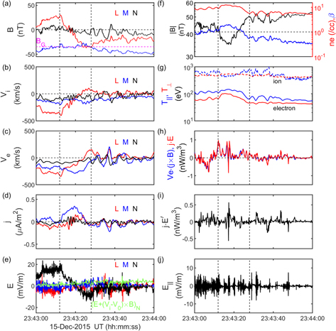
Figure 1. (a)–(g) MMS1 observations of a large guide-field reconnection X-line during the magnetopause crossing enclosed by the vertical lines, with vectors shown in LMN coordinate systems. (h)–(j) The rates of energy conversion and the parallel electric fields. The magenta dashed line in panel (a) denotes the ambient reconnection guide field. The green line in panel (e) denotes the Hall electric fields evaluated in the X-line moving frame.
Download figure:
Standard image High-resolution imageAs indicated in Figure 1(e), the Hall electric fields evaluated in the X-line moving frame,  , were pointing toward the magnetosheath side within the magnetopause, similar to the results shown in Figure 6(d) of Pritchett & Mozer (2009) for asymmetric reconnection with a guide field. The Hall magnetic field, BM
− BG
, was positive for the quadrants (ViL
< 0, BL
>0) and (ViL
>0, BL
< 0), as shown in Figure 1(a). A remarkable feature was observed in the β > 1 region (β is the ratio of the ion thermal pressure to the magnetic pressure; see Figure 1(f)), namely, that low-frequency waves were found in both the magnetic field and ion velocity components in the
L
and
N
directions. These waves were also seen at the current densities jL
and jN
. Later, it will be demonstrated that changes in BL
and BN
were negatively correlated with those for the ion plasma velocity. Furthermore, low-frequency waves were also found in the ion and electron velocities in the low β region (β < 1). The rates of energy conversion,
j
·
E
,
V
e
· (
j
×
B
), and
, were pointing toward the magnetosheath side within the magnetopause, similar to the results shown in Figure 6(d) of Pritchett & Mozer (2009) for asymmetric reconnection with a guide field. The Hall magnetic field, BM
− BG
, was positive for the quadrants (ViL
< 0, BL
>0) and (ViL
>0, BL
< 0), as shown in Figure 1(a). A remarkable feature was observed in the β > 1 region (β is the ratio of the ion thermal pressure to the magnetic pressure; see Figure 1(f)), namely, that low-frequency waves were found in both the magnetic field and ion velocity components in the
L
and
N
directions. These waves were also seen at the current densities jL
and jN
. Later, it will be demonstrated that changes in BL
and BN
were negatively correlated with those for the ion plasma velocity. Furthermore, low-frequency waves were also found in the ion and electron velocities in the low β region (β < 1). The rates of energy conversion,
j
·
E
,
V
e
· (
j
×
B
), and  , are shown in Figures 1(h) and (i), where
  . The dot product of
  can be written as
j
·
E
−
V
e
· (
j
×
B
), where
V
e
· (
j
×
B
) is the rate of work done by the Lorentz force in the ideal MHD. Therefore, the nonzero
can be written as
j
·
E
−
V
e
· (
j
×
B
), where
V
e
· (
j
×
B
) is the rate of work done by the Lorentz force in the ideal MHD. Therefore, the nonzero  indicates the nonideal MHD energy transfer between electromagnetic fields and plasmas (Zenitani et al. 2012). One can find in Figure 1(j) that significant parallel electric fields were present during the energy conversion process.
In Figure 2 each component of the magnetic field vector in LMN coordinates was plotted on top of the corresponding component of - V i and - V e , together with a color map of the electron pitch angle distribution (PAD) for energy range 0.2–2.0 keV. It is seen that changes in B were negatively correlated with V i and V e . Field-aligned counter-streaming electrons were detected within the magnetopause, which is considered one of the signatures for the reconnection ion diffusion region (e.g., Teh et al. 2012). Changes in BL and BN were mostly coupled with -ViL and -ViN within the magnetopause, while in the upstream region, the magnetic field variations were coupled with both the ion and electron velocities for all three components.

Figure 2. (a) Electron PAD for the energy range of 0.2–2.0 keV. (b)–(d) The overlaid plots of the magnetic field and the ion and electron velocity (− V i and − V e ) for each component in LMN coordinate systems. The vertical lines mark the duration of the magnetopause crossing.
Download figure:
Standard image High-resolution imageBy calculating the consecutive differences in
V
i
(δ
V
i
), the wave structures of
V
i
were manifested and then compared with δ
V
a
= δ(
B
/ ), as shown in Figures 3(a)–(c). Here
V
a
is the ion Alfvén velocity, mp
is the proton mass, and n is the plasma density. For the time interval enclosed by the green lines in Figures 3(a)–(c), the δ
V
i
perturbations were negatively correlated with δ
V
a
and dominant at the
L
and
N
directions. The slope of a regression line was ∼−1.3 between δ
ViL and δ
VaL and ∼−1.6 between δ
ViN and δ
VaN, while these two slopes became −0.3 and −0.7 for the time interval enclosed by the gray lines. Comparisons of δ
V
e
with δ
V
a
in Figures 3(d)–(f) revealed that the δ
V
e
perturbations were also negatively correlated with δ
V
a
in between the gray lines, but not found in between the green lines. The δ
V
e
perturbations were present at all three components, where the regression slopes were −0.6, −1.3, and −0.6 for the
L
,
M
, and
N
directions, respectively. In the next section, it will be shown that the first waveform is of an SAW and the other is of a KAW. Figure 3(g) compares the Poynting flux magnitude, ∣S∣, with the parallel one, ∣S∥∣, and indicates that the wave Poynting flux parallel to the magnetic field carries most of the energy, expected for SAW and KAW. The ratios Te∥/Te⊥ and T∥/T⊥ show that the parallel temperature for ions and electrons was increased at KAW (Figure 3(h)). It is noteworthy that the peaks of T∥/T⊥ were located near the wave peaks denoted by the red dashed lines, while the peaks of Te∥/Te⊥ were near the wave troughs.
), as shown in Figures 3(a)–(c). Here
V
a
is the ion Alfvén velocity, mp
is the proton mass, and n is the plasma density. For the time interval enclosed by the green lines in Figures 3(a)–(c), the δ
V
i
perturbations were negatively correlated with δ
V
a
and dominant at the
L
and
N
directions. The slope of a regression line was ∼−1.3 between δ
ViL and δ
VaL and ∼−1.6 between δ
ViN and δ
VaN, while these two slopes became −0.3 and −0.7 for the time interval enclosed by the gray lines. Comparisons of δ
V
e
with δ
V
a
in Figures 3(d)–(f) revealed that the δ
V
e
perturbations were also negatively correlated with δ
V
a
in between the gray lines, but not found in between the green lines. The δ
V
e
perturbations were present at all three components, where the regression slopes were −0.6, −1.3, and −0.6 for the
L
,
M
, and
N
directions, respectively. In the next section, it will be shown that the first waveform is of an SAW and the other is of a KAW. Figure 3(g) compares the Poynting flux magnitude, ∣S∣, with the parallel one, ∣S∥∣, and indicates that the wave Poynting flux parallel to the magnetic field carries most of the energy, expected for SAW and KAW. The ratios Te∥/Te⊥ and T∥/T⊥ show that the parallel temperature for ions and electrons was increased at KAW (Figure 3(h)). It is noteworthy that the peaks of T∥/T⊥ were located near the wave peaks denoted by the red dashed lines, while the peaks of Te∥/Te⊥ were near the wave troughs.
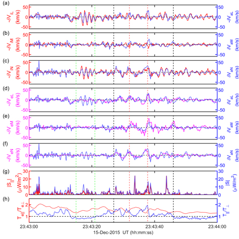
Figure 3. (a)–(f) Wave structures for ion and electron plasma velocities, and magnetic field. (g) Comparison of the Poynting flux ∣S∣ to ∣S∥∣. (h) The ratio of parallel to perpendicular temperature for ions (blue) and electrons (red). The first and second waveforms are enclosed by the green and gray lines, respectively. The red dashed lines denote the wave peaks.
Download figure:
Standard image High-resolution image3. Wavevector Analysis
Figure 4(a) shows for the four MMS spacecraft the δ
BL
of the first waveform in the time interval between 23:43:15 and 23:43:21 UT, where the high-frequency fluctuations in δ
BL
have been removed by the Savitzky–Golay filter with a span width of 91 data points. One can see that the crossing times of the wavefront for the four spacecraft were different. Figure 4(b) shows the power spectral density (PSD) of δ
BL
based on MMS1. A single spectral peak, denoted by the red dashed line, was present at fm
= ∼0.74 Hz, smaller than the proton gyrofrequency fci (green line), in the spacecraft frame. Using a bandpass filter at 0.70–0.78 Hz, a single-frequency wave can be approximately derived. Therefore, the wavevector,
k
, and the wave phase speed, vph, can be estimated by the multi-spacecraft timing method, where
m
= ( ) =
) =  and ∣
k
∣ = 1. Here κα
is the reciprocal vector for the spacecraft tetrahedron (Chanteur 1998) and tγ
α
= tα
− tγ
is the crossing time difference between two spacecraft, where tγ
is at the reference spacecraft, which is MMS1 in this study. The time delays tγ
α
were determined by the maximum value of the cross-correlation function. The timing analysis results for the first waveform were vph =
and ∣
k
∣ = 1. Here κα
is the reciprocal vector for the spacecraft tetrahedron (Chanteur 1998) and tγ
α
= tα
− tγ
is the crossing time difference between two spacecraft, where tγ
is at the reference spacecraft, which is MMS1 in this study. The time delays tγ
α
were determined by the maximum value of the cross-correlation function. The timing analysis results for the first waveform were vph =  = 281 km s−1 and
k
= vph
m
= (−0.491, −0.816, 0.304) (GSE). A wave normal angle θBk of ∼18° formed between
k
and the magnetic field and the ratio of k⊥ to k∥ was ∼0.3. Since the magnetic X-line is moving southward (V0z
<0) and kz
> 0, the wave is thus propagating away from the diffusion region. The wavenumber, k, can then be roughly estimated as 2
= 281 km s−1 and
k
= vph
m
= (−0.491, −0.816, 0.304) (GSE). A wave normal angle θBk of ∼18° formed between
k
and the magnetic field and the ratio of k⊥ to k∥ was ∼0.3. Since the magnetic X-line is moving southward (V0z
<0) and kz
> 0, the wave is thus propagating away from the diffusion region. The wavenumber, k, can then be roughly estimated as 2  = 1.644 × 10⁻² km−1, which gives k⊥
d = ∼0.2. Here d = ∼41 km is the ion thermal gyroradius based on upstream values of T⊥ = 410 eV and B = 50 nT. In the ion velocity frame of reference, the wave frequency was estimated as fps
=
= 1.644 × 10⁻² km−1, which gives k⊥
d = ∼0.2. Here d = ∼41 km is the ion thermal gyroradius based on upstream values of T⊥ = 410 eV and B = 50 nT. In the ion velocity frame of reference, the wave frequency was estimated as fps
=  = ∼0.41 Hz = ∼0.118 fci, where
  = (−115.8, −119.8, −95.5) (km s−1) is the average ion plasma velocity. In summary, the overall result suggests that the first waveform is of an SAW, in terms of the parallel wave propagation,
  <1, and k⊥
d <1.
<1, and k⊥
d <1.
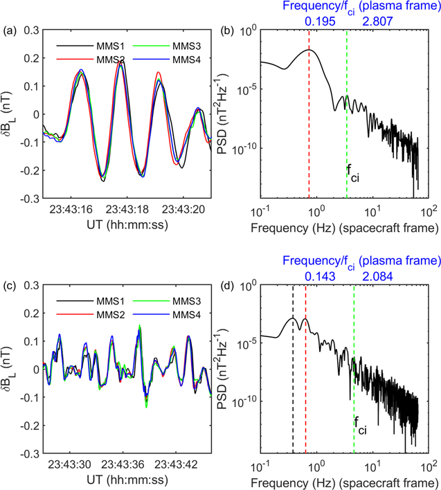
Figure 4. The consecutive difference in BL at the four MMS spacecraft for (a) SAW and (c) KAW. The PSD of δ BL based on MMS1 is displayed for (b) SAW and (d) KAW, where the red and black dashed lines denote the spectral peaks, and the proton gyrofrequency is at the green line. The two values of the normalized frequency correspond to 1 Hz and 10 Hz in the spacecraft frame.
Download figure:
Standard image High-resolution imageFigure 4(c) shows the δ
BL
of the second waveform for the four spacecraft in the time interval between 23:43:27 and 23:43:46 UT. In Figure 4(d), two spectral peaks with comparable PSD were present at fm1 = ∼0.38 Hz (black dashed line) and fm2 = ∼0.64 Hz (red dashed line) in the spacecraft frame. A single-frequency wave can approximately be extracted for fm1 and fm2, by using a bandpass filter at 0.35–0.40 Hz and 0.6–0.7 Hz, respectively. For fm1, vph1 = 120 km s−1 and
k
1 = (−0.272, −0.222, 0.936) (GSE), with θBk = ∼80o and  = ∼5.6. For fm2, vph2 = 170 km s−1 and
k
2 = (−0.739, −0.230, 0.633) (GSE), with θBk = ∼67° and
= ∼5.6. For fm2, vph2 = 170 km s−1 and
k
2 = (−0.739, −0.230, 0.633) (GSE), with θBk = ∼67° and  = ∼2.3. The resulting wavenumbers for fm1 and fm2 are k1 = 1.962 × 10⁻² km−1 and k2 = 2.362 × 10⁻² km−1, giving k⊥
d = 0.8 and 0.9, respectively. The wave frequencies in the ion velocity frame, i.e.,
= ∼2.3. The resulting wavenumbers for fm1 and fm2 are k1 = 1.962 × 10⁻² km−1 and k2 = 2.362 × 10⁻² km−1, giving k⊥
d = 0.8 and 0.9, respectively. The wave frequencies in the ion velocity frame, i.e.,  = (−56.8, −72.1, 48.5) (km s−1), were fps1 = ∼0.13 Hz = ∼0.029 fci and fps2 = ∼0.30 Hz = ∼0.066 fci. Note that the normalized frequency in the plasma frame in Figure 4(d) was calculated using the
k
2 result. Apparently, the second waveform is different than the SAW seen in the magnetopause layer. It is suggested that the second waveform is of a KAW, in terms of the perpendicular propagation, k⊥/k∥ > 1, and k⊥
d ∼ 1. Since k1z
and k2z
are directed northward, the KAW is thus propagating away from the reconnection site.
= (−56.8, −72.1, 48.5) (km s−1), were fps1 = ∼0.13 Hz = ∼0.029 fci and fps2 = ∼0.30 Hz = ∼0.066 fci. Note that the normalized frequency in the plasma frame in Figure 4(d) was calculated using the
k
2 result. Apparently, the second waveform is different than the SAW seen in the magnetopause layer. It is suggested that the second waveform is of a KAW, in terms of the perpendicular propagation, k⊥/k∥ > 1, and k⊥
d ∼ 1. Since k1z
and k2z
are directed northward, the KAW is thus propagating away from the reconnection site.
Additionally, the wave dispersion relation was examined for SAW and KAW, using the multi-spacecraft timing method developed by Zhang et al. (2022), where the phase speed and wavevector were calculated at each time for each single-frequency wave in the range from zero to the Nyquist frequency. In Figures 5(a) and (c), the dispersion relations are shown for θBk = 0°–30° (SAW) and θBk = 60°–90° (KAW), where the color code denotes the wave power P(f, k) derived from a wavelet transform and the red dashed line denotes the local Alfvén speed. As compared to SAW, the KAW has a much wider k range at the same frequency, suggesting the presence of multiple wave branches in the KAW. The frequency versus k⊥ d is also shown for SAW (Figure 5(b)) and KAW (Figure 5(d)). In Figure 5, the cross and triangle symbols denote the previous analysis results for SAW and KAW. A good agreement is found at the cross symbols, where at the same wave frequency the result of the cross symbol is close to the one with a high wave power, but a large discrepancy at the triangle symbol. This discrepancy could be attributed to the multiple wave branches in KAW.

Figure 5. The dispersion relation and frequency vs. k⊥ d for (a), (b) SAW and (c), (d) KAW. The color code is the wave power derived from a wavelet transform. The red dashed line in (a) and (c) denotes the local Alfvén speed at 221 and 394 km s−1, respectively. The cross and triangle results are obtained from a different method.
Download figure:
Standard image High-resolution image
4. Summary and Discussion
A large guide-field (∼1.1Bo) reconnection X-line, observed by the MMS spacecraft during the outbound magnetopause crossing, has been examined for Alfvén waves. The current sheet thickness of the magnetopause was ∼2.6 ion inertial lengths (∼269 km), where the field-aligned counter-streaming electrons were detected and the Hall electromagnetic fields were identified. An SAW was present in the magnetopause layer. Remarkably, a KAW was seen in the magnetopause upstream region after an SAW was encountered. Low-frequency magnetic field fluctuations were negatively correlated with the changes in the ion and electron velocities at KAW, but only in the ion velocity at SAW. The wavevector
k
was predicted by the multi-spacecraft timing method using four-point magnetic field measurements. The timing analysis results of  , k⊥
d, and the wave propagation direction were satisfied for both the KAW and SAW. In the spacecraft frame, the wave frequency was ∼0.74 Hz for SAW and ∼0.38 Hz/∼0.64 Hz for KAW. The parallel Poynting flux carried most of the wave energy in the KAW and SAW, away from the reconnection site. The parallel temperature for ions and electrons was increased at KAW and the peaks of T∥/T⊥ for ions were located near the wave peaks, while the ratio peaks for electrons were near the wave troughs.
, k⊥
d, and the wave propagation direction were satisfied for both the KAW and SAW. In the spacecraft frame, the wave frequency was ∼0.74 Hz for SAW and ∼0.38 Hz/∼0.64 Hz for KAW. The parallel Poynting flux carried most of the wave energy in the KAW and SAW, away from the reconnection site. The parallel temperature for ions and electrons was increased at KAW and the peaks of T∥/T⊥ for ions were located near the wave peaks, while the ratio peaks for electrons were near the wave troughs.
It is unexpected that the perturbed fields of the SAW are not correlated with the electron velocity variations. During the SAW time interval, strong field-aligned, counter-streaming electrons were present (Figure 2(a)). This will lead to a non-Maxwellian distribution in the phase space density. Moreover, the calculated electron bulk velocity is significantly smaller than the electron thermal speed (∼4400 km s−1). One may speculate that the electron bulk velocity may not be accurately estimated. Thus, this result needs to be interpreted with caution.
The flow speed of the plasma frame is distinct between SAW and KAW, where the SAW was observed in the faster plasma frame. In the spacecraft frame, the wave frequency (∼0.74 Hz) of the SAW is fairly close to that of the KAW at ∼0.64 Hz, and their Doppler shifts ( ) are fairly consistent (∼0.34 Hz). Since the SAW was in the faster plasma frame as compared to the KAW, the wavelength of the SAW is expected to be larger than that of the KAW.
The magnetic energy of the Hall magnetic fields is believed to be propagating away from the reconnection site by Alfvén waves. It has been demonstrated in simulations that the Hall magnetic field structures are carried away by KAWs (Shay et al. 2011). From a 2D kinetic simulation of magnetotail reconnection with zero guide field, Gurram et al. (2021) showed that magnetic reconnection can generate both SAWs and KAWs when an ion-to-electron mass ratio of 400 and open boundary conditions were implemented and that the SAWs can become the main carrier of wave energy during reconnection. In this studied event, both SAW and KAW were detected near the reconnection X-line, suggesting that KAWS and SAWs can be generated by asymmetric reconnection with a large guide field.
Acknowledgments
This work was supported by the grants of Universiti Kebangsaan Malaysia (GP-2021-K020730 and GP-K020730). W.L.T. thanks Stein Haaland for providing a list of magnetopause crossings by MMS. Special thanks to the dedicated efforts of the entire MMS mission team for data access. MMS data can be downloaded at the NASA CDAWeb at http://cdaweb.gsfc.nasa.gov/.