


Abstract
We perform a 2.5-dimensional particle-in-cell simulation of a quasi-parallel shock, using parameters for the Earth's bow shock, to examine electron acceleration and heating due to magnetic reconnection. The shock transition region evolves from the ion-coupled reconnection dominant stage to the electron-only reconnection dominant stage, as time elapses. The electron temperature enhances locally in each reconnection site, and ion-scale magnetic islands generated by ion-coupled reconnection show the most significant enhancement of the electron temperature. The electron energy spectrum shows a power law, with a power-law index around 6. We perform electron trajectory tracing to understand how they are energized. Some electrons interact with multiple electron-only reconnection sties, and Fermi acceleration occurs during multiple reflections. Electrons trapped in ion-scale magnetic islands can be accelerated in another mechanism. Islands move in the shock transition region, and electrons can obtain larger energy from the in-plane electric field than the electric potential in those islands. These newly found energization mechanisms in magnetic islands in the shock can accelerate electrons to energies larger than the achievable energies by the conventional energization due to the parallel electric field and shock drift acceleration. This study based on the selected particle analysis indicates that the maximum energy in the nonthermal electrons is achieved through acceleration in ion-scale islands, and electron-only reconnection accounts for no more than half of the maximum energy, as the lifetime of sub-ion-scale islands produced by electron-only reconnection is several times shorter than that of ion-scale islands.
Export citation and abstract BibTeX RIS

Original content from this work may be used under the terms of the Creative Commons Attribution 4.0 licence. Any further distribution of this work must maintain attribution to the author(s) and the title of the work, journal citation and DOI.
1. Introduction
In situ spacecraft observations in the Earth's bow shock and the magnetosheath (the downstream region of the bow shock), such as by Cluster and Magnetospheric Multiscale (MMS), have shown that there are many current sheets embedded within the shock-driven turbulence where magnetic reconnection actively converts magnetic energy into particle kinetic and thermal energies (Retinò et al. 2007; Yordanova et al. 2016; Vörös et al. 2017; Phan et al. 2018; Gingell et al. 2019; Wang et al. 2019; Stawarz et al. 2022). In a turbulent plasma, magnetic fields are stirred, field lines are complexly entangled, and, as a result, some reconnection sites are embedded within small regions whose size is of the order of several ion skin depths. In those regions, MMS observations revealed a novel type of magnetic reconnection—electron-only reconnection—where only electrons are participating in reconnection, while ions are just passing through the reconnection region because ions cannot respond to such small-scale magnetic gradients (Phan et al. 2018).
Electron-only reconnection has been observed by MMS in the Earth's magnetosheath (Phan et al. 2018; Stawarz et al. 2019, 2022; Gingell et al. 2021), the transition region in the Earth's bow shock (Chen et al. 2019; Gingell et al. 2019, 2020; Wang et al. 2019), the foreshock region (Liu et al. 2020; Wang et al. 2020), and the early stage of magnetic reconnection in the Earth's magnetotail (Lu et al. 2020). Numerical studies by 2.5-dimensional particle-in-cell (PIC) simulations (Bessho et al. 2022) show that the reconnection outflows accelerated by electron-only reconnection in shock turbulence can reach of the order of the electron Alfvén speed, which is the square root of the ion-to-electron mass ratio  times larger than the outflow speed in the standard ion-coupled reconnection (around the Alfvén speed). As a result, the convection electric field due to the electron outflow,
E
= −
V
e,out ×
B
/c, is also much greater than that in the standard reconnection. Note that the region around the peak of the electron outflow speed is where electrons start to be magnetized, and the magnetic field lines and the electron fluid move together. The reconnection electric field, which is the electric field at the reconnection X line, balances with the convection electric field due to the outflow. Hence, the reconnection electric field also becomes
times larger than the outflow speed in the standard ion-coupled reconnection (around the Alfvén speed). As a result, the convection electric field due to the electron outflow,
E
= −
V
e,out ×
B
/c, is also much greater than that in the standard reconnection. Note that the region around the peak of the electron outflow speed is where electrons start to be magnetized, and the magnetic field lines and the electron fluid move together. The reconnection electric field, which is the electric field at the reconnection X line, balances with the convection electric field due to the outflow. Hence, the reconnection electric field also becomes  times larger than that in the standard reconnection, and we expect that significant particle acceleration due to electron-only reconnection in turbulent regions occurs.
Full PIC and hybrid PIC simulations (Karimabadi et al. 2014; Matsumoto et al. 2015; Bohdan et al. 2017, 2020; Gingell et al. 2017, 2023; Bessho et al. 2019, 2020, 2022; Lu et al. 2021; Ng et al. 2022) show magnetic reconnection in the shock-driven turbulence, and ion-coupled reconnection can also occur where both ion and electron jets are produced. Ion-coupled reconnection has been observed by MMS (Yordanova et al. 2016; Vörös et al. 2017; Wang et al. 2019; Stawarz et al. 2022) in the magnetosheath and the transition region of the Earth's bow shock. Our previous simulation study (Bessho et al. 2020) found a link between ion-coupled reconnection in a shock and the ion–ion beam instability. It is known that ions reflected by a quasi-parallel shock can travel toward the upstream region, and electromagnetic waves are produced due to the interaction between the reflected ions and the incident ions (see PIC simulation studies of quasi-parallel shocks by Kato 2015 and Otsuka et al. 2019, where the waves excited by the resonant instability propagate toward the upstream region in the upstream rest frame, and the wavelength is several tens of ion inertial lengths). Our previous study, Bessho et al. (2020), also showed that reflected ions flow into the upstream region, exciting large-amplitude electromagnetic waves. The waves are generated by a nonresonant ion–ion beam instability in the shock transition region (Sentman et al. 1981; Gary et al. 1984; Gary 1991; Wilson 2016), which is called the Bell instability (Bell 2004; Weidl et al. 2019) in astrophysical shocks when the nonresonant mode is generated by cosmic rays. In our previous PIC simulation study, where the Alfvén Mach number is around 11, the wavelength of the excited waves is around a few ion inertial lengths, and the waves propagate toward the shock in the upstream rest frame (opposite to the direction observed by Kato 2015 and Otsuka et al. 2019). The magnetic field lines are bent due to the excited nonresonant waves, and ion-coupled reconnection occurs to produce ion-scale (several ion-skin-depth size) magnetic flux ropes. The timescale of ion-coupled reconnection (several ion cyclotron periods) is much longer than the timescale of electron-only reconnection, which was observed to be a fraction of the ion cyclotron period in the simulations. In contrast, simulation studies (Bessho et al. 2020, 2022) also show that the number of electron-only reconnection sites is much lager than that of ion-coupled reconnection sites. Therefore, it is important to investigate the cumulative effect of the energy dissipation by electron-only reconnection compared with ion-coupled reconnection in shocks, and how the shock dynamics is affected by both types of reconnection, which generate heat and enhance the pressure in the shock.
Both types of reconnection are expected to generate energetic particles in shocks, but how important these reconnection sites are in the total shock heating has not been addressed yet. MMS observations show electron heating in reconnecting current sheets in the transition region of the Earth's bow shock (Wang et al. 2019). Also, in the foreshock region in the Earth's bow shock and Mars, solitary magnetic structures (called short large-amplitude magnetic structures) are generated by nonresonant ion–ion instability (Chen et al. 2021, 2022), which eventually can cause reconnection and heat electrons (Wang et al. 2020). In this study, performing a 2.5-dimensional PIC simulation of a quasi-parallel shock, we elucidate how reconnection (both electron-only and ion-coupled reconnection) energizes and heats electrons, and we compare other electron energization mechanisms in a shock such as acceleration due to the electrostatic field associated with the cross-shock potential (Woods 1969; Goodrich & Scudder 1984; Scudder 1995), and shock drift acceleration (Holman & Pesses 1983; Wu 1984; Ball & Melrose 2001).
In Section 2, we describe the simulation method. In Section 3, we show simulation results of a quasi-parallel shock, both types of reconnection, and electron acceleration and heating in the shock. In Section 4, we give conclusions of this study.
2. Simulation Method
We perform a 2.5-dimensional, electromagnetic, relativistic, PIC simulation for a quasi-parallel shock. The simulation domain has the initial uniform magnetic field ![${{\boldsymbol{B}}}_{0}=[{B}_{0}\cos \theta ,{B}_{0}\sin \theta ,0]$](https://content.cld.iop.org/journals/0004-637X/954/1/25/revision1/apjace321ieqn3.gif) , where θ is the shock normal angle. The ion and electron densities are also uniform, ni
= ne
= n0. We impose a uniform electric field
, where θ is the shock normal angle. The ion and electron densities are also uniform, ni
= ne
= n0. We impose a uniform electric field  , which can provide a uniform plasma drift speed vd
in the negative x-direction. Note that we use cgs units in the simulation, and the electric field is measured based on B0. At time t = 0, all of the particles have a drift speed in the negative x-direction with a speed vd
. The x = 0 boundary is a conducting wall, and particles are specularly reflected. From the x = Lx
boundary, new particles are injected, and the field boundary condition is also a conducting wall. The boundaries in y-direction are periodic boundaries. We use the system size Lx
× Ly
= 1000di
× 25.6di
, where di
is the ion skin depth based on the density n0. The shock normal angle is 25°, the ion-to-electron mass ratio mi
/me
is 200, the ratio of the plasma frequency ωpe
(based on n0) to the electron cyclotron frequency Ωe
(based on B0) is 4, and the beta values for ions and electrons are βi
= βe
= 1. The particle injection speed vd
= 9.0vA0, where vA0 is the Alfvén speed based on B0 and n0. Note that this Alfvén speed is nonrelativistic,
, which can provide a uniform plasma drift speed vd
in the negative x-direction. Note that we use cgs units in the simulation, and the electric field is measured based on B0. At time t = 0, all of the particles have a drift speed in the negative x-direction with a speed vd
. The x = 0 boundary is a conducting wall, and particles are specularly reflected. From the x = Lx
boundary, new particles are injected, and the field boundary condition is also a conducting wall. The boundaries in y-direction are periodic boundaries. We use the system size Lx
× Ly
= 1000di
× 25.6di
, where di
is the ion skin depth based on the density n0. The shock normal angle is 25°, the ion-to-electron mass ratio mi
/me
is 200, the ratio of the plasma frequency ωpe
(based on n0) to the electron cyclotron frequency Ωe
(based on B0) is 4, and the beta values for ions and electrons are βi
= βe
= 1. The particle injection speed vd
= 9.0vA0, where vA0 is the Alfvén speed based on B0 and n0. Note that this Alfvén speed is nonrelativistic,  , and much smaller than the electron thermal speed,
  . The ion sound speed is
  , where Γ = 5/3 is the specific heat ratio, and Ti
and Te
are the ion and electron temperatures, respectively. The speed of the fast mode wave is
, where Γ = 5/3 is the specific heat ratio, and Ti
and Te
are the ion and electron temperatures, respectively. The speed of the fast mode wave is ![${v}_{f}={\left\{{v}_{{\rm{A}}0}^{2}+{c}_{s}^{2}+{[{({v}_{{\rm{A}}0}^{2}+{c}_{s}^{2})}^{2}-4{v}_{{\rm{A}}0}^{2}{c}_{s}^{2}{\cos }^{2}\theta ]}^{1/2}\right\}}^{1/2}/{2}^{1/2}=1.4{v}_{{\rm{A}}0}$](https://content.cld.iop.org/journals/0004-637X/954/1/25/revision1/apjace321ieqn8.gif) , and the injection speed vd
= 9.0vA0 corresponds to 6.4vf
. The number of particles per cell per species is 100. Note that these simulation parameters are identical to the ones used in the previous papers (Bessho et al. 2019, 2020, 2022), except for Lx
and Ly
, where Lx
( = 1000di
) is longer than the previous one (Lx
= 375di
), while Ly
( = 25.6di
) is halved from the previous one (Ly
= 51.2di
). We use Lx
larger than the one used in the previous studies, to reduce the effect of the boundary at x = Lx
that might affect the physics in the shock.
, and the injection speed vd
= 9.0vA0 corresponds to 6.4vf
. The number of particles per cell per species is 100. Note that these simulation parameters are identical to the ones used in the previous papers (Bessho et al. 2019, 2020, 2022), except for Lx
and Ly
, where Lx
( = 1000di
) is longer than the previous one (Lx
= 375di
), while Ly
( = 25.6di
) is halved from the previous one (Ly
= 51.2di
). We use Lx
larger than the one used in the previous studies, to reduce the effect of the boundary at x = Lx
that might affect the physics in the shock.
3. Simulation Results
3.1. Shock Propagation and Reconnection Regions
Figure 1 shows the time evolution of the shock between Ωi t = 18.75 to 21.88, where Ωi is the ion cyclotron frequency based on B0. The black curves in panels (a), (b), and (c) are magnetic field lines projected on the x–y plane, and the color indicates the out-of-plane current density Jz . As time progresses, many kinetic-scale (up to several di ) magnetic islands are generated in the shock transition region (the region right of the white vertical line). The white vertical line in each plot is the position of the maximum of 〈By 〉 (see the arrows in panel (d)), where 〈By 〉 is the magnetic field By averaged over the y-direction. Based on the propagation of the peak of 〈By 〉, we determine that the shock speed during this time interval is 1.5vA0 in the simulation frame. Considering the upstream drift speed 9vA0, the shock speed vsh in the upstream rest frame is 10.5vA0, i.e., the Alfvén Mach number MA is 10.5, and the fast mode Mach number Mf = vsh/vf is 7.5. At Ωi t = 18.75 (see panel (a)), there are several ion-scale magnetic islands whose size is several di , for example, around (x, y) = (49di , 0), (47di , 12di ), and (46di , 22di ), each of which is denoted by 1, 2, and 3, respectively, in the plot. They are generated because of the nonresonant ion–ion beam instability (Sentman et al. 1981; Gary et al. 1984; Gary 1991; Bessho et al. 2020; Chen et al. 2021, 2022). More details about the nonresonant wave as well as the resonant wave observed in the simulation are summarized in Appendix A. Many thin current sheets are generated, with both positive and negative Jz . These ion-scale magnetic islands grow further as time elapses, and at Ωi t = 20.31 (panel (b)), the size of islands at (x, y) = (45di , 7di ) (island 1) and (x, y) = (46di , 20di ) (island 2) becomes greater than that at Ωi t = 18.75. Note that the magnetic islands 1, 2, and 3 at Ωi t = 20.31 are the same islands 1, 2, and 3 at Ωi t = 18.75, respectively. At Ωi t = 20.31, around those ion-scale islands, there are many sub-di scale (several de -scale, where de is the electron skin depth) magnetic islands. These are electron-only reconnection sties, in which electron jets form but ions just pass through the region without significant acceleration because of the small scale of magnetic gradients in these thin current sheets. The formation of these electron-only reconnection regions was discussed in the previous paper (Bessho et al. 2020). At Ωi t = 21.88 (panel (c)), the ion-scale larger islands have already been dissipated (i.e., they merge surrounding fields, and the X lines associated with those islands disappear), and only smaller electron-only reconnection areas remain in a region 46di < x < 50di .

Figure 1. (a)–(c) Time evolution of current density Jz . Black curves are magnetic field lines. The white vertical line in each plot shows the position of the maximum 〈By 〉 (the y average of By ), which roughly indicates the position of the shock plane. Three ion-scale magnetic islands are denoted by numbers 1–3. (d) Profiles of 〈By 〉, which is By averaged over y. The arrows show the same positions of the white line in each of panels (a)–(c). (e) 2D field lines at Ωi t = 20.31, and two lines, y = 20di and y = 18di , along which 1D cuts of By are shown in panel (f). The position of an X line is denoted by X. (f) 1D cuts of By along y = 20di (thick blue) and y = 18di (black). The thin blue curve shows 〈By 〉.
Download figure:
Standard image High-resolution imagePanel (f) shows 1D cuts of By along two lines, y = 20di and y = 18di at Ωi t = 20.31 (see also panel (e)). The line y = 20di crosses the ion-scale island (island 2), while the line y = 18di passes through two sub-di scale islands. In panel (f), the thick blue curve is the 1D cut along y = 20di . By is positive in the left side of the island (x < 46di ), and By reverses its sign across the center of the island (x = 46di ) and becomes negative in the right side of the island (46di < x). This island covers the region 44.5di < x < 47.3di (see the blue arrow), and the size of this island (diameter) is around 3di . Across the island, By changes from 7B0 to −5B0. The black curve in panel (f) shows the 1D cut along y = 18di , which crosses the two sub-di scale islands. The two sub-di scale islands are denoted by black arrows in panel (f) (see also panel (e)). Across these two islands, By changes its sign, and the change of By is from 6B0 to −4B0, which is similar to the change of By in the ion-scale island. The size of these islands is smaller than di . Left of these sub-di scale islands, there is a reconnection X line (see also panel (e), where the X line is marked by "X"), and By also changes its sign across the X line region (i.e., a current sheet). The current sheet thickness is also around di . In panel (f), the thin blue curve represents the y-averaged value, 〈By 〉 (the same blue curve as in panel (d)). Compared with 〈By 〉, the local 1D cuts show larger-amplitude fluctuations.
Figure 2 shows the y-component of the ion and electron fluid velocities Viy
and Vey
at Ωi
t = 20.31, near the region of an ion-scale magnetic island (island 2). We focus on two X lines: at (x, y) = (45.475di
, 18.45di
) (see the blue X mark) and (x, y) = (46.825di
, 18.925di
) (see the red X mark). The blue X line is in the reconnection region that generates the ion-scale magnetic island (island 2), where ion-coupled reconnection occurs. In panel (a), we see that an ion outflow jet (marked by the black oval) is generated because of reconnection with the blue X line, while panel (b) shows that an electron outflow jet is also produced along the separatrix. Both the ion and electron outflows are generated on the upper-left side of the separatrix with Viy
> 0 and Vey
> 0, and there are no downward (with Viy
< 0 and Vey
< 0) outflows in the lower right side of the separatrix. Formation of such a one-sided outflow jet (in this case, a flow with positive-y velocity) is a characteristic in turbulent reconnection in a shock (Bessho et al. 2022), and the ion outflow velocity (the velocity measured in the simulation frame, not the velocity relative to the plasma surrounding the jet) exceeds 6vA0, while the electron outflow reaches 10vA0, which is close to the electron Alfvén speed vAe0 under the mass ratio 200 (vAe0 = 14.4vA0). The local values of magnetic fields (let us denote them as B1 and B2) and densities (n1 and n2) in the two sides across the current sheet around the blue X line are: B1 = 5.6B0, B2 = 2.7B0, n1 = 3.0n0, and n2 = 2.7n0, which give the local Alfvén speed, vA-local = 3.2vA0 (using B1 and n1) and 1.6vA0 (using B2 and n2), respectively. The theoretical estimate of the ion outflow speed based on the asymmetric reconnection model (Cassak & Shay 2007), ![${V}_{\mathrm{out}}={[{B}_{1}{B}_{2}({B}_{1}+{B}_{2})/4\pi {m}_{i}({n}_{1}{B}_{2}+{n}_{2}{B}_{1})]}^{1/2}$](https://content.cld.iop.org/journals/0004-637X/954/1/25/revision1/apjace321ieqn9.gif) , is obtained as 2.3vA0, which is close to the local Alfvén speeds, but is much smaller than the observed ion outflow speed ∼6vA0. Note that the ion outflow generated by reconnection in the shock transition region can exceed the Alfvén speed, reaching of the order of 10vA0, because of the super-Alfvénic background ion flows in the shock transition region (Bessho et al. 2022). In contrast, the red X line at (x, y) = (46.825di
, 18.925di
) is a site of electron-only reconnection, and the ion plot (panel (a)) does not have an ion outflow jet from the red X line, while the electron plot (panel (b)) shows a rightward electron outflow jet that exceeds 10vA0 (see the black oval around the red X line).
, is obtained as 2.3vA0, which is close to the local Alfvén speeds, but is much smaller than the observed ion outflow speed ∼6vA0. Note that the ion outflow generated by reconnection in the shock transition region can exceed the Alfvén speed, reaching of the order of 10vA0, because of the super-Alfvénic background ion flows in the shock transition region (Bessho et al. 2022). In contrast, the red X line at (x, y) = (46.825di
, 18.925di
) is a site of electron-only reconnection, and the ion plot (panel (a)) does not have an ion outflow jet from the red X line, while the electron plot (panel (b)) shows a rightward electron outflow jet that exceeds 10vA0 (see the black oval around the red X line).
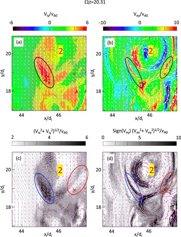
Figure 2. Contours of the y-component of the ion fluid velocity Viy
and the electron fluid velocity Vey
. Magenta lines are magnetic field lines. Island 2 is the same ion-scale island as in Figure 1. The blue X mark and the red X mark show the positions of reconnection X lines associated with ion-coupled reconnection and electron-only reconnection, respectively. In panels (a) and (b), the regions with black ovals are where jets are generated. White arrows show the velocity vectors. (c) In grayscale, the in-plane speed of ion fluid,  is shown. (d) In grayscale, the in-plane speed of electron fluid,
  , multiplied by the sign of Vey
is shown. Only the regions with positive Vey
are shown in grayscale, and the regions with negative Vey
are in white. In both panels (c) and (d), magenta arrows represent the fluid velocity vectors, and the blue and red oval regions are around the blue X line and the red X line, respectively.
, multiplied by the sign of Vey
is shown. Only the regions with positive Vey
are shown in grayscale, and the regions with negative Vey
are in white. In both panels (c) and (d), magenta arrows represent the fluid velocity vectors, and the blue and red oval regions are around the blue X line and the red X line, respectively.
Download figure:
Standard image High-resolution imagePanels (c) and (d) display the in-plane speeds of the ions and the electrons. Panel (c) shows the ion in-plane speed,  , and only the regions with Viy
> 2vA0 are shown in grayscale. Let us denote the two X lines as (x, y) = (xX1, yX1) (blue X line) and (x, y) = (xX2, yX2) (red X line). Around the blue X line, ions are flowing into the reconnection site from the region y < yX1. The inflow speed at the blue X line is around 5vA0, and in the outflow region (within the blue oval), the maximum speed exceeds 6.5vA0. In contrast, the ion in-plane speed around the red X line does not constitute the outflow jet. Around the red X line, ions are passing through the red X line from the region xX2 < x and y < yX2 with velocities Vix
< 0 and Viy
> 0 (see the vector plot with magenta arrows). The ion in-plane flows are perpendicular to the magnetic field reversal (i.e., the current sheet), and they are decelerated (see the change of the color from gray to white after passing through the magnetic field reversal). After passing through this magnetic field reversal region, the ion flows are deflected by the magnetic field gradient in the ion-scale island, and the flow velocity changes to Vix
∼ 0 and Viy
> 0. During this deflection, the ion in-plane flow speed is a bit enhanced (see the gray region around x = 47di
and x = 20di
), and this increase may be due to the local electric fields (the detailed acceleration mechanism is beyond the scope of this paper). However, there is no collimated ion jet structure produced from the red X line, indicating that the increase of the ion speed is not due to the formation of a reconnection outflow jet. In contrast, the ion jet forms from the blue X line, and it shows a conspicuous collimated jet structure. The size of island 2, which is generated by the reconnection region with the blue X line, is larger than 2di
, while the size of the magnetic islands generated by electron-only reconnection with the red X line is less than di
. Ions may be slightly affected by the small-size islands in the electron-only reconnection region, but the change of ion speed is not substantial, and no ion jet forms. In contrast, around the red X line, a strong electron jet is seen whose speed exceeds 10vA0 (panel (d)). More details for ion-coupled reconnection regions and electron-only reconnection regions in 2D PIC simulations are discussed in Bessho et al. (2019, 2020, 2022).
, and only the regions with Viy
> 2vA0 are shown in grayscale. Let us denote the two X lines as (x, y) = (xX1, yX1) (blue X line) and (x, y) = (xX2, yX2) (red X line). Around the blue X line, ions are flowing into the reconnection site from the region y < yX1. The inflow speed at the blue X line is around 5vA0, and in the outflow region (within the blue oval), the maximum speed exceeds 6.5vA0. In contrast, the ion in-plane speed around the red X line does not constitute the outflow jet. Around the red X line, ions are passing through the red X line from the region xX2 < x and y < yX2 with velocities Vix
< 0 and Viy
> 0 (see the vector plot with magenta arrows). The ion in-plane flows are perpendicular to the magnetic field reversal (i.e., the current sheet), and they are decelerated (see the change of the color from gray to white after passing through the magnetic field reversal). After passing through this magnetic field reversal region, the ion flows are deflected by the magnetic field gradient in the ion-scale island, and the flow velocity changes to Vix
∼ 0 and Viy
> 0. During this deflection, the ion in-plane flow speed is a bit enhanced (see the gray region around x = 47di
and x = 20di
), and this increase may be due to the local electric fields (the detailed acceleration mechanism is beyond the scope of this paper). However, there is no collimated ion jet structure produced from the red X line, indicating that the increase of the ion speed is not due to the formation of a reconnection outflow jet. In contrast, the ion jet forms from the blue X line, and it shows a conspicuous collimated jet structure. The size of island 2, which is generated by the reconnection region with the blue X line, is larger than 2di
, while the size of the magnetic islands generated by electron-only reconnection with the red X line is less than di
. Ions may be slightly affected by the small-size islands in the electron-only reconnection region, but the change of ion speed is not substantial, and no ion jet forms. In contrast, around the red X line, a strong electron jet is seen whose speed exceeds 10vA0 (panel (d)). More details for ion-coupled reconnection regions and electron-only reconnection regions in 2D PIC simulations are discussed in Bessho et al. (2019, 2020, 2022).
Figure 3 displays the electric fields Ex , Ey , and Ez in the same region as Figure 1 at the three times. In the shock, there are three types of electric fields: one is the electrostatic field associated with the cross-shock potential (Woods 1969; Goodrich & Scudder 1984; Scudder 1995). This electric field is mainly in the x-direction, and Ex > 0. The second type of electric field is generated in ion-scale magnetic islands, and this electric field points toward the center of each island. The third type of electric field is the reconnection electric field, and in this 2D simulation, this electric field is in the z-direction.

Figure 3. Contours of electric fields: (a)–(c) Ex , (d)–(f) Ey , and (g)–(i) Ez . Black curves are magnetic field lines. In ion-scale islands, there are strong in-plane electric fields (Ex and Ey ) pointing to the center of each island.
Download figure:
Standard image High-resolution imageOverall, Ex (panels (a), (b), and (c)) in the shock transition region is positive, and this Ex > 0 causes the formation of the cross-shock potential. In addition to that, there are local enhancements of the magnitude of Ex due to the formation of turbulence and reconnection areas. In the ion-scale magnetic islands, Ex becomes positive in the left side of the islands, while Ex becomes negative in the right side of the islands. Panels (d), (e), and (f) for Ey show that the top part of each ion-scale island has negative Ey , while the bottom part has positive Ey . In summary, the in-plane electric fields in each ion-scale magnetic island are pointing toward the center. The magnitude of the in-plane electric field in those islands reaches B0.
These strong in-plane electric fields inside the ion-scale islands are considered to be the Hall electric field, because they are generated by the convection effect, E in-plane = − Vez e z × B /c, where e z is the z-component unit vector. Since ∣Viz ∣ ≪ ∣Vez ∣ in these regions, Jz ∼ − enVez holds, and E in-plane ∼ Jz e z × B /(ene c). As we will see later in Sections 3.2 and 3.3, these Hall electric fields in the ion-scale islands play an important role to energize electrons. Note that the Hall electric field E Hall = J × B /c cannot be a source for a net energy increase in the total plasma, because J · E Hall = 0. However, it can transfer the energy from one species to another, such as from ions to electrons. Let us estimate the magnitude of the in-plane electric field, considering the convection electric field Ex = Vez By /c. Since electrons are accelerated to reach the electron Alfvén speed, Vez in the ion-scale island also becomes of the order of vAe0. Therefore, Vez /c ∼ vAe0/c = Ωe /ωpe = 1/4 in the simulation, and we obtain Ex ∼ Vez By /c ∼ B0 using By ∼ 4B0, which is the magnetic field in the shock (see Figure 1(d)). In a spacecraft observation, if the magnetic field and the plasma density in the solar wind are B0 = 5 nT and n0 = 20 cm−3, respectively (consistent with typical observation values such as in Gingell et al. 2017, 2019; Wang et al. 2019), the electric field Ex in an island would be 4cB0(Ωe /ωpe ) ∼ 20 mV m−1.
In a 1D laminar shock model, the Ez
component is a constant value across the shock, with its magnitude  under the initial parameters in this study. However, in the 2D simulation, the shock transition region becomes highly turbulent, and panels (g), (h), and (i) of Figure 3 show that there are locally enhanced positive and negative Ez
in the shock transition region. At Ωi
t = 18.75 (panel (g)), there are positive and negative stripes of Ez
mostly along the ion-scale magnetic islands. The convection electric field is given by Ez
= − Vex
By
/c + Vey
Bx
/c, and the electron fluid velocities in this region are basically Vex
< 0 and Vey
> 0 (not shown, but see Figure 1 in Bessho et al. 2019). The top-left side of an ion-scale island (the second quadrant of the island with respect to the island center) has positive Ez
, because Bx
> 0 and By
> 0. In contrast, the bottom-right side of the island (the fourth quadrant of the island) shows negative Ez
, because Bx
< 0 and By
< 0. At Ωi
t = 20.31 (panel (h)), several sub-ion-scale islands are generated due to electron-only reconnection, and there are local enhancements of positive and negative Ez
in those regions. The polarity of Ez
varies from island to island, because the electron fluid velocities vary in each sub-ion-scale island. At Ωi
t = 21.88 (panel (i)), after those ion-scale islands are dissipated, the intensity of Ez
becomes smaller than the previous times in panels (g) and (h).
under the initial parameters in this study. However, in the 2D simulation, the shock transition region becomes highly turbulent, and panels (g), (h), and (i) of Figure 3 show that there are locally enhanced positive and negative Ez
in the shock transition region. At Ωi
t = 18.75 (panel (g)), there are positive and negative stripes of Ez
mostly along the ion-scale magnetic islands. The convection electric field is given by Ez
= − Vex
By
/c + Vey
Bx
/c, and the electron fluid velocities in this region are basically Vex
< 0 and Vey
> 0 (not shown, but see Figure 1 in Bessho et al. 2019). The top-left side of an ion-scale island (the second quadrant of the island with respect to the island center) has positive Ez
, because Bx
> 0 and By
> 0. In contrast, the bottom-right side of the island (the fourth quadrant of the island) shows negative Ez
, because Bx
< 0 and By
< 0. At Ωi
t = 20.31 (panel (h)), several sub-ion-scale islands are generated due to electron-only reconnection, and there are local enhancements of positive and negative Ez
in those regions. The polarity of Ez
varies from island to island, because the electron fluid velocities vary in each sub-ion-scale island. At Ωi
t = 21.88 (panel (i)), after those ion-scale islands are dissipated, the intensity of Ez
becomes smaller than the previous times in panels (g) and (h).
To see the overall structures in the electric fields and magnetic fields in the shock transition region, let us discuss quantities averaged over y and examine their 1D structures. In the following, a quantity 〈Q〉 represents the field quantity Q averaged over y. Panels (a)–(c) in Figure 4 display the three components of the electric field, 〈Ex 〉, 〈Ey 〉, and 〈Ez 〉, as a function of x, while panel (d) shows the magnetic field 〈Bz 〉. For 〈By 〉, see Figure 1(d). Note that 〈Bx 〉 is a constant, because 〈∇ · B 〉 = 〈dBx /dx〉 = 0, and 〈Bx 〉 is not plotted in Figure 4. Panel (a) shows 〈Ex 〉, and at Ωi t = 18.75, the peak is around 0.25B0 at x = 44di . At Ωi t = 20.31, the peak increased a lot, and the value is around 0.45B0 at x = 48di . There is a secondary peak 0.38B0 at x = 45di , and the dip between the highest and the secondary peaks is due to the growth of ion-scale magnetic islands. At Ωi t = 21.88, the peak moves farther to the right, and the peak value is around 0.3B0 at x = 49.5di . The smaller peak value is because the ion-scale islands have already been dissipated at Ωi t = 21.88. Overall, 〈Ex 〉 > 0 in the shock transition region, which makes the cross-shock potential positive. Panel (b) is for 〈Ey 〉, and it is positive in the region where 〈Ex 〉 is very small (such as x > 50di ), while 〈Ey 〉 is negative in the region where 〈Ex 〉 becomes large. 〈Ey 〉 is mostly determined by the convection electric field, Ey = − Vez Bx /c + Vex Bz /c. In the region with strong 〈Ex 〉, electrons move with the Ex × By drift in the positive z-direction; therefore, the first term, −Vez Bx /c, dominates, and Ey becomes negative. In contrast, in the region where 〈Ex 〉 is small (x > 50di ), there is a finite negative 〈Bz 〉 (see panel (d)), and the second term, Vex Bz /c, becomes large because Vex < 0 and Bz < 0, which makes Ey positive.

Figure 4. Profiles of y-averaged quantities. (a) 〈Ex 〉, (b) 〈Ey 〉, (c) 〈Ez 〉, and (d) 〈Bz 〉. 〈Ex 〉 is positive in the shock transition region, forming a large cross-shock potential. 〈Ez 〉 is fluctuating around the upstream value 0.067B0. 〈Bz 〉 becomes negative in the shock transition region.
Download figure:
Standard image High-resolution imagePanel (c) shows that overall, 〈Ez
〉 is positive because of the motional electric field  however, in the shock transition region, 〈Ez
〉 fluctuates because of waves and generation of magnetic islands. In the far-upstream region in x > 70di
(not shown), 〈Ez
〉 asymptotes to the value 0.067B0. Panel (d) demonstrates that 〈Bz
〉 becomes negative, and this is because the electron drift Vez
> 0 drags the magnetic field line in the shock transition region. Therefore, a large-magnitude 〈Bz
〉 ∼ − 4B0 is generated, and reconnection in this region becomes guide field reconnection in 2D simulations (Bessho et al. 2019, 2020, 2022). Note that in 3D cases (see Ng et al. 2022), the reconnection plane does not have to be in the x–y plane; therefore, reconnection can occur with a small guide field if the reconnection plane rotates and it becomes close to the x–z plane.
however, in the shock transition region, 〈Ez
〉 fluctuates because of waves and generation of magnetic islands. In the far-upstream region in x > 70di
(not shown), 〈Ez
〉 asymptotes to the value 0.067B0. Panel (d) demonstrates that 〈Bz
〉 becomes negative, and this is because the electron drift Vez
> 0 drags the magnetic field line in the shock transition region. Therefore, a large-magnitude 〈Bz
〉 ∼ − 4B0 is generated, and reconnection in this region becomes guide field reconnection in 2D simulations (Bessho et al. 2019, 2020, 2022). Note that in 3D cases (see Ng et al. 2022), the reconnection plane does not have to be in the x–y plane; therefore, reconnection can occur with a small guide field if the reconnection plane rotates and it becomes close to the x–z plane.
These electric fields, both the in-plane fields (Ex and Ey ) and the out-of-plane field Ez (partially due to the reconnection electric field), are important to energize and heat electrons in the shock. In the next subsection, we will discuss electron acceleration and heating.
3.2. Electron Heating in the Shock Transition Region due to Reconnection
Figure 5 illustrates the time evolution of the electron temperature Te
. In the shock upstream region (x > 60di
, not shown in the figure), the electron temperature is  . In Figure 5, the shock transition region is shown, and Te
already increases from the far-upstream value. As time progresses, the number of reconnection sites (also the number of magnetic islands) is getting larger and larger. As a result, the electron temperature is also increasing with time in the region 44 < x/di
< 50. Both X lines and magnetic islands show the temperature enhancement, and the temperature in the entire region 40 < x/di
< 50 also increases (the background color changes from green,
. In Figure 5, the shock transition region is shown, and Te
already increases from the far-upstream value. As time progresses, the number of reconnection sites (also the number of magnetic islands) is getting larger and larger. As a result, the electron temperature is also increasing with time in the region 44 < x/di
< 50. Both X lines and magnetic islands show the temperature enhancement, and the temperature in the entire region 40 < x/di
< 50 also increases (the background color changes from green,  , to yellow,
  ). Note that Te
is defined as
). Note that Te
is defined as ![$\left[1/(3{n}_{e})\right]{m}_{e}{\sum }_{j}\int {f}_{e}{({v}_{j}-{V}_{ej})}^{2}{d}^{3}v$](https://content.cld.iop.org/journals/0004-637X/954/1/25/revision1/apjace321ieqn18.gif) , where ne
is the electron density, fe
is the distribution function, vj
is the j-component of an electron velocity, and the sum is over the three components j = x, y, and z. The temperature Te
represents the thermal energy based on the entire distribution function fe
; however, as discussed in Goldman et al. (2020), when there are multiple beam components in fe
, this definition of Te
represents a mixture of real thermal energy (based on the random speed with respect to each beam velocity) and a pseudo-thermal energy (the energy due to a relative velocity with respective to the bulk fluid velocity, and this can be nonzero even in the limit of cold beams). The temperature Te
can increase either due to the production of multiple beams, or the actual heating associated with the increase of random thermal spread, or both.
, where ne
is the electron density, fe
is the distribution function, vj
is the j-component of an electron velocity, and the sum is over the three components j = x, y, and z. The temperature Te
represents the thermal energy based on the entire distribution function fe
; however, as discussed in Goldman et al. (2020), when there are multiple beam components in fe
, this definition of Te
represents a mixture of real thermal energy (based on the random speed with respect to each beam velocity) and a pseudo-thermal energy (the energy due to a relative velocity with respective to the bulk fluid velocity, and this can be nonzero even in the limit of cold beams). The temperature Te
can increase either due to the production of multiple beams, or the actual heating associated with the increase of random thermal spread, or both.

Figure 5. (a)–(c) Time evolution of electron temperature Te . Ion-scale islands 1–3 are the same as those in Figure 1. Te becomes large in ion-scale islands (panel (b)). After those ion-scale islands are dissipated (panel (c)), Te still shows large values. (d) Energy spectra at these three times, in log–log scale, obtained in the x-interval marked by the red horizontal bar under the x-axis in each time. The horizontal red bar in panels (a), (b), and (c) covers the region 43 < x/di < 45 (panel (a)), 45 < x/di < 47 (panel (b)), and 47 < x/di < 49 (panel (c)). (e) The same energy distributions as in panel (d), but in log-linear scale. In panels (d) and (e), black curves are spectra in the upstream region, at x = 500di . Nonthermal electrons are generated, and the spectra show a power law, with an index around 6.
Download figure:
Standard image High-resolution imageAt Ωi t = 18.75 (panel (a)), the electron temperature is mostly uniform (green color) throughout the region; however, an ion-scale island (denoted by 2 in the plot) and a small-size island (indicated by a blue arrow) have local enhancements of Te (yellow and red color). Also, around x = 44di , there are several stripes of red and yellow colors. Both island 1 and island 3 show no temperature enhancement yet. At Ωi t = 20.31 (panel (b)), there are three ion-scale magnetic islands (islands 1, 2, and 3) with significantly enhanced Te . Small-scale islands, which are produced due to electron-only reconnection, also show high Te (red color), but some small-scale islands still show lower temperatures (yellow color). At this time, the ion-scale large islands are the dominant electron energization sites. In contrast, at Ωi t = 21.88 (panel (c)), the large ion-scale islands have already been dissipated, and the red regions with high temperatures spread throughout the y-direction in the region 46di < x < 49di . Later (in Figures 7 and 8), we will see that the increase of Te in magnetic islands is associated with multiple beams.
Figures 5(d) and (e) display the electron energy spectra at the three different times. Panel (d) is a log–log plot, while panel (e) is a linear-log plot, using the same distribution functions. Green, blue, and red curves are the energy spectra obtained at three different times, plot (a), (b), and (c), respectively, in the region marked by the red bar in the horizontal axis in each panel. The marked spatial interval at each time covers regions with significant temperature enhancements. At Ωi
t = 18.75, nonthermal electrons are produced (see the green curve in panel (e), and compare with the black curve, which is the upstream electron distribution at x = 500di
). In panel (d), the energy spectrum at Ωi
t = 18.75 (green) already shows a power-law-like distribution, and if we approximate the green curve as a power-law function, the power-law index is close to 6.0. Let us define εK
as εK
= γ − 1, where γ is the Lorentz factor, and εK
represents the kinetic energy normalized by me
c2. The average of εK
at Ωi
t = 18.75 is 0.32 (this value, εK
= γ − 1 = 0.32, corresponds to  , and v/vTe-up = 2.6, where v is a speed, and vTe-up is the upstream electron thermal speed
  ). At Ωi
t = 20.31, when the ion-scale islands show the most significant electron temperature enhancements, the average of εK
becomes 0.47, and panels (d) and (e) show that the electrons at Ωi
t = 20.31 (blue) are significantly energized compared with the electrons at Ωi
t = 18.75 (green). At Ωi
t = 21.88, when the ion-scale islands were already dissipated, the maximum energy in the spectrum (red) becomes smaller than that at the previous time Ωi
t = 20.31, suggesting that the most significant energization occurs at Ωi
t = 20.31 because of the ion-scale islands. In contrast, the average of εK
at Ωi
t = 21.88 is 0.52, and it continuously increases from Ωi
t = 20.31 to Ωi
t = 21.88, suggesting that electrons are continuously accelerated during the dissipation of the ion-scale islands and due to electron-only reconnection that generates small-scale islands. All three curves (green, blue, and red) in panel (d) show that the power-law indices do not significantly change between Ωi
t = 18.75 and 20.31, and they are close to 6.
). At Ωi
t = 20.31, when the ion-scale islands show the most significant electron temperature enhancements, the average of εK
becomes 0.47, and panels (d) and (e) show that the electrons at Ωi
t = 20.31 (blue) are significantly energized compared with the electrons at Ωi
t = 18.75 (green). At Ωi
t = 21.88, when the ion-scale islands were already dissipated, the maximum energy in the spectrum (red) becomes smaller than that at the previous time Ωi
t = 20.31, suggesting that the most significant energization occurs at Ωi
t = 20.31 because of the ion-scale islands. In contrast, the average of εK
at Ωi
t = 21.88 is 0.52, and it continuously increases from Ωi
t = 20.31 to Ωi
t = 21.88, suggesting that electrons are continuously accelerated during the dissipation of the ion-scale islands and due to electron-only reconnection that generates small-scale islands. All three curves (green, blue, and red) in panel (d) show that the power-law indices do not significantly change between Ωi
t = 18.75 and 20.31, and they are close to 6.
Choosing an X line and a magnetic island, we investigated the time evolution of the local temperatures and electron distribution functions. In Figure 6, the magenta closed circles are on the X line (position A), while the cyan circles are inside the island (position B). Both positions A and B demonstrate enhancements of the local temperatures as time elapses. At position A (X line) at Ωi
t = 18.75, the temperature is  (green color in panel (a)), and it increases to
  (red color in panel (c)) at Ωi
t = 19.38 because of reconnection. After this time, the magnetic island above this X line (its island center is around x = 45.7di
and y = 10di
) becomes smaller and smaller, and at Ωi
t = 19.69, the X line and the island have already disappeared. We chose two positions at Ωi
t = 19.69: position A and position A', which are not on an X line, but at positions in a red color region in panel (d), corresponding to the region where previously there an X line at Ωi
t = 19.38. The electron temperature Te
at position A (at (x, z) = (45.0di
, 9.5di
)) is
(red color in panel (c)) at Ωi
t = 19.38 because of reconnection. After this time, the magnetic island above this X line (its island center is around x = 45.7di
and y = 10di
) becomes smaller and smaller, and at Ωi
t = 19.69, the X line and the island have already disappeared. We chose two positions at Ωi
t = 19.69: position A and position A', which are not on an X line, but at positions in a red color region in panel (d), corresponding to the region where previously there an X line at Ωi
t = 19.38. The electron temperature Te
at position A (at (x, z) = (45.0di
, 9.5di
)) is  , while Te
at position A' (at (x, z) = (45.0di
, 10di
)) is
, while Te
at position A' (at (x, z) = (45.0di
, 10di
)) is  .
.
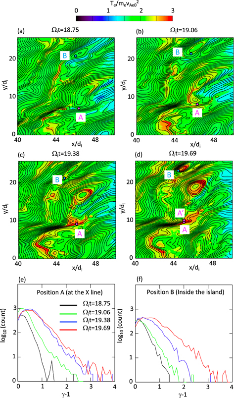
Figure 6. (a)–(d) Time evolution of electron temperature Te . The magenta point (A) is the position of an X line, while the cyan point (B) is inside an ion-scale island. (e)–(f) Electron energy spectra at position A (panel(e)) and position B (panel (f)). At Ωi t = 19.69 (panel (d)), there is no X line around position A, and the magnetic island above position A seen in panel (c) has already been dissipated in panel (d). Two positions, A and A', are chosen in the region where Te is large (red color region).
Download figure:
Standard image High-resolution imagePosition B (magnetic island) also shows Te
increase as time elapses. At Ωi
t = 18.75, the temperature is  . The temperature gradually enhances, and at Ωi
t = 19.38, it becomes
. The temperature gradually enhances, and at Ωi
t = 19.38, it becomes  . It continues to rise, and at Ωi
t = 19.69, Te
reaches
. It continues to rise, and at Ωi
t = 19.69, Te
reaches  . In the island, the temperature becomes large around the outer boundary of the island, and the center of the island has a smaller temperature than the outer region. Panel (d) shows a few ion-scale islands, and the electron temperature has a similar ring-like structure inside the islands, where the high-temperature region surrounds the central low temperature region.
Panels (e) and (f) in Figure 6 are the electron energy distribution functions at those two positions A and B. To compose these distribution functions, we collected electrons in a square region with a size 0.1di × 0.1di around each position. At position A (X line), the energy distribution function shows an increase in its width (the FWHM for the peak) until Ωi t = 19.38. The highest εK ( = γ − 1) is around 1 at Ωi t = 18.75 (black curve), while the highest energy εK exceeds 4 at Ωi t = 19.69 (the highest εK is 5.1, not shown). Note that the spectrum for position A' at Ωi t = 19.69 is similar to that for position A, and we only plotted the spectrum at position A in panel (e). At position B (magnetic island, panel (f)), significant electron energization occurs between Ωi t = 19.38 (blue curve) and 19.69 (red curve). The energy distribution at Ωi t = 19.69 (red curve) shows a slightly harder spectrum than those at position A. The highest εK at Ωi t = 19.69 is 5.7 (not shown).
Figure 7 demonstrates the time evolution of the electron distribution function at position A. Panels (a)–(c) are reduced distribution functions in 2D velocity planes, integrated over the third direction (for example, panel (a) is the 2D reduced distribution function in the vx
–vy
plane, integrated over vz
). At position A, at Ωi
t = 18.75 (Te
= 2.0me
vAe0), the electron distribution function is nongyrotropic (panels (a)–(c)), where the white lines in panels (b) and (c) represent the direction of the magnetic field. Note that there is only Bz
at the X line; therefore, panel (a) for the velocity plane vx
–vy
does not show the direction of the magnetic field, and this vx
–vy
plane is the velocity plane perpendicular to the magnetic field. The phase space densities in the regions of vx
> 0, vy
> 0, and vz
< 0 become high. As time evolves, reconnection generates heated electrons, and at Ωi
t = 19.06 (panels (d)–(f)), the gyrotropy of the distribution function increases and regions with high phase space density (red regions) spread. At this time, the temperature becomes  . At Ωi
t = 19.38 (panels (g)–(i)), the radius of the distribution function becomes larger than that at the previous time, and the temperature increases to Te
∼ 3.0me
vAe0. At this time, multiple electron beams are seen in each velocity plane. In particular, panel (i) in the vz
–vx
plane shows two major components: the component with vz
< 0 and vx
> 0 and the component with vz
> 0 and vx
∼ 0. After the X line is dissipated, at Ωi
t = 19.69 (panels (j)–(l)), the radius of the distribution function does not significantly change, suggesting that the electron temperature also does not significantly change after Ωi
t = 19.38, but the distributions show a notable change from the previous time. Panels (k) and (l) show a strong electron beam moving in the positive vz
-direction. Panels (m)–(o) are for the distributions at position A', which is close to position A. There are still multiple electron beams, but the thermal spread in panels (m)–(o) for position A' (
. At Ωi
t = 19.38 (panels (g)–(i)), the radius of the distribution function becomes larger than that at the previous time, and the temperature increases to Te
∼ 3.0me
vAe0. At this time, multiple electron beams are seen in each velocity plane. In particular, panel (i) in the vz
–vx
plane shows two major components: the component with vz
< 0 and vx
> 0 and the component with vz
> 0 and vx
∼ 0. After the X line is dissipated, at Ωi
t = 19.69 (panels (j)–(l)), the radius of the distribution function does not significantly change, suggesting that the electron temperature also does not significantly change after Ωi
t = 19.38, but the distributions show a notable change from the previous time. Panels (k) and (l) show a strong electron beam moving in the positive vz
-direction. Panels (m)–(o) are for the distributions at position A', which is close to position A. There are still multiple electron beams, but the thermal spread in panels (m)–(o) for position A' ( ) is more significant than that in panels (j)–(l) for position A (
 ). At position A', the z-directional beam component in panel (o) can be seen, but the red part spread in the region −20vA0 < vz
< 45vA0, which is more spread than that in panel (l) for position A, where the red region is more localized in a region 20vA0 < vz
< 45vA0. This indicates that the z-directional beam is dissipating in a lower vz
region, and electron heating is occurring. We conclude that some high-temperature regions contain multiple electron beams, and those high-speed beams play important roles for electron heating. Detailed mechanisms about how electron beams are scattered to heat electrons are beyond the scope of this paper.
). At position A', the z-directional beam component in panel (o) can be seen, but the red part spread in the region −20vA0 < vz
< 45vA0, which is more spread than that in panel (l) for position A, where the red region is more localized in a region 20vA0 < vz
< 45vA0. This indicates that the z-directional beam is dissipating in a lower vz
region, and electron heating is occurring. We conclude that some high-temperature regions contain multiple electron beams, and those high-speed beams play important roles for electron heating. Detailed mechanisms about how electron beams are scattered to heat electrons are beyond the scope of this paper.

Figure 7. (a)–(l) Reduced 2D electron distribution functions at position A (X line), shown in Figure 6. Panels (a)–(c) are distribution functions at Ωi t = 18.75, and the white lines in panels (b) and (c) show the direction of the magnetic field. Panel (a) shows the velocity plane perpendicular to the magnetic field. As time evolves, the temperature (thermal spread) increases, and multiple beams are generated. (m)–(o) Electron distributions at position A' in Figure 6. Compared with panels (j)–(l) for position A, the thermal spread around each of multiple beams is larger, suggesting that heating occurs.
Download figure:
Standard image High-resolution imageFigure 8 shows the time evolution of the electron distribution function at position B (magnetic island). At time Ωi t = 18.75 (panels (a)–(c)), the distribution function is nongyrotropic, but compared with the distribution at position A (panels (a)–(c) in Figure 7), the distribution at point B is more gyrotropic. As time evolves, the radius of the distribution function increases. Panels (d)–(f) at Ωi t = 19.06 show that the radius of the distribution is slightly larger than at the previous time. The increase of the radius of the distribution function continues until Ωi t = 19.69. At the same time of the increase of the radius, a strong z-directional electron beam is generated at Ωi t = 19.38 (panels (g)–(i)), and the beam remains until Ωi t = 19.69 (panels (j)–(l)). Again, the beam formation is one of the causes of the electron temperature enhancement in the magnetic island. Compared with the distribution at the X line (Figure 7), the distribution in the island has a persistent strong electron beam that lasts longer than the beam at the X line. Note that the beam direction is not parallel to the magnetic field. This z-directional electron beam can be understood as the beam generated by the E × B drift due to the in-plane electric fields Ex and Ey . As we have seen in Figure 3, in each ion-scale island, there is a strong Hall electric field that points toward the center of the island. Magnetized electrons are drifting in the positive z-direction because of the E × B drift due to the in-plane electric fields in each island, and even unmagnetized energetic electrons can drift in the same direction as the E × B drift; therefore, we observe the strong z-directional beam in panels (h), (i), (k), and (l) in Figure 8.
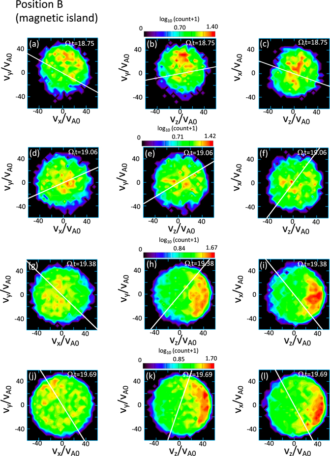
Figure 8. Reduced 2D electron distribution functions at position B (magnetic island), shown in Figure 6. White lines show the direction of the magnetic field. As time evolves, the temperature (thermal spread) increases, and at the same time, a strong z-directional beam is generated.
Download figure:
Standard image High-resolution image3.3. Electron Acceleration and Particle Tracing
We investigate individual electrons' trajectories to understand where and how they are accelerated in the shock transition region. We choose electrons (actual particles in the PIC simulation, not test particles) in regions where reconnection occurs, and trace their trajectories and the time evolution of their momenta, energies, and the work done by each component of electric field, which is given by −e∫Ej vj dt, where j represents a component of the electric field, either j = x, y, or z, or j = ∥ (parallel to B ), and the perpendicular work is defined as the total work subtracted by the parallel work.
We plot in Figure 9 the trajectory of an electron that is accelerated at an X line denoted by X1 (at (x, y) = (46di , 7.5di )) in panel (a) at Ωi t = 18.91. The black curves are magnetic field lines, and the particle trajectory starting at Ωi t = 18.75 is shown by the red curve. In panel (a), among several X lines in this plot, two reconnection X lines, X1 and X2, are marked. X1 is the same X line as position A in Figure 6. The electron is interacting with X1, and it is ejected to the outflow region left of the X line. Panel (d) is the time evolution of the electron's Lorentz factor γ, and γ − 1 represents the kinetic energy normalized by me c2. The electron's γ is increasing at Ωi t = 18.75 up to 1.8, and after the ejection, it decreases a little bit to 1.5 at Ωt = 18.91. Panel (b) displays the trajectory until Ωi t = 19.31. The X line is moving upward during the time interval between Ωi t = 18.91 and 19.31. After the electron was ejected from X1 at Ωi t = 18.91, it moves downstream to the left of X1, but the electron is reflected in the downstream region and returns back to X1 again at Ωi t = 19.31. During the second interaction with X1 (after Ωi t = 19.2), the electron gets accelerated and gains energy. Panels (e) and (f) are the time evolution of the work done by the perpendicular and the parallel electric fields, and the perpendicular and the parallel momenta of this particle, respectively. (The vertical axis scale in panels (d), (e), and (f) is chosen as the same scale as in Figure 10 for another electron, which shows more dramatic changes of these quantities than this electron in Figure 9.) In panel (d), the Lorentz factor γ becomes almost constant until Ωi t = 19.2, and after that time, it continuously increases with time until Ωi t = 19.6. Panel (e) displays the work done by the perpendicular electric field (red) and the parallel electric field (blue). During the interval between Ωi t = 19.31 and Ωi t = 19.6, the energy increase is due to the perpendicular electric field. Panel (c) shows the particle trajectory until Ωi t = 19.69, and this particle is moving back and forth in the y-direction after Ωi t = 19.31, during the interaction with X1. The magnetic island between X1 and X2 is gradually dissipated between Ωi t = 19.31 and 19.69, and X1 has already disappeared at Ωi t = 19.69 (panel (c)). Panel (f) shows the momentum components: the perpendicular momentum (red) and the parallel momentum (blue). During the time interval between Ωi t = 19.31 and Ωi t = 19.6, the parallel momentum p∥ changes its sign five times, during which the perpendicular momentum p⊥ is slightly increasing. Both ∣p⊥∣ and ∣p∥∣ are increasing during the bounce motion. This acceleration resembles Fermi acceleration, but the parallel momentum increase is less significant than the increase of p⊥, except for at the time of the final reversal of p∥ around Ωi t = 19.6. After Ωi t = 19.6, the electron is ejected to the downstream region with negative p∥.
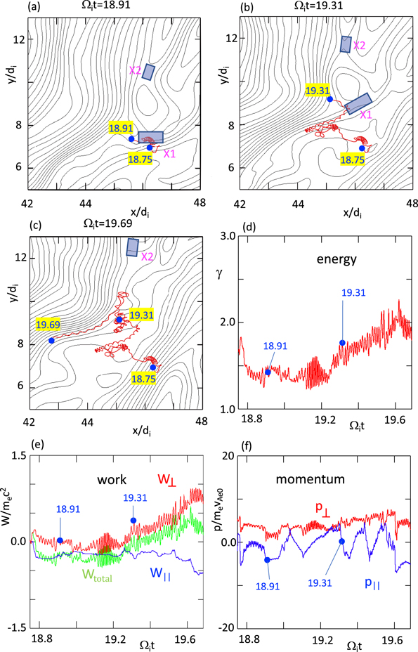
Figure 9. (a)–(c) (Red) The trajectory of an electron in the x–y plane. (Black) Magnetic field lines. X1 and X2 denote the locations of X lines. (d) Time evolution of the Lorentz factor γ. (e) Time evolution of the work done by the perpendicular electric field (W⊥ in red), the work done by the parallel electric field (W∥ in blue), and the sum of these two (Wtotal in green). (f) Time evolution of the perpendicular momentum (p⊥ in red) and the parallel momentum (p∥ in blue).
Download figure:
Standard image High-resolution image
Figure 10. (a)–(c) The trajectory of another electron. (d)–(f) Time evolution of γ, W⊥, W∥, Wtotal, p⊥, and p∥. Panels (a)–(f) are in the same format as in Figure 9. This electron shows clear signatures of Fermi acceleration. (g) Evolution of γ in the y–γ plane. The positions of X3 and X5 are shown by the vertical dashed lines. Each color shows a segment in each bounce motion, either from right to left or from left to right (denoted by R → L or L → R). At each bounce motion, γ increases. (h) γ as a function of time. Each color corresponds to the time interval in each segment shown in panel (g).
Download figure:
Standard image High-resolution imageFigure 10 shows the trajectory of another electron. In panel (a), we see that this electron is moving back and forth between two X lines, X3 and X4. At Ωi t = 19.06, the Lorentz factor γ is around 1.75 (see panel (d)). After Ωi t = 19.06, the energy starts to increase, and γ reaches 2.5. Panel (e) indicates that the energy increase is due to the perpendicular work, and both γ and W⊥ have step-function-like enhancements, consistent with the physical picture of Fermi acceleration, where the energy enhancement occurs due to each bounce motion, as we see in the following. Panel (b) illustrates that during the bounce motion between X3 and X4, another X line (X5) forms between X3 and X4. Then this electron is trapped between X3 and X5, and starts to bounce between X3 and X5. The Lorentz factor γ continues to increase during the bounce motion between X3 and X5, between Ωi t = 19.35 and 19.58. Panel (f) demonstrates that the parallel momentum p∥ changes its sign during the bounce motion, and the magnitude of p∥ increases at each bounce. This step-function-like increase of γ, energization due to the perpendicular electric field, and the increase of ∣p∥∣ are signatures of Fermi acceleration in contracting islands (Drake et al. 2006).
To see the details of this Fermi acceleration, we plot the dependence of the Lorentz factor γ on the y-position in Figure 10(g), during the multibounce motion between X3 and X5 between Ωi t = 19.35 and 19.58. The locations of the two X lines, X3 and X 5 are denoted by the vertical dashed lines. Each color in the curve corresponds to the segment during a certain time interval. For example, the magenta curve is the segment during 19.35 < Ωi t < 19.40, when the particle is moving from right to left (denoted as R → L). During this time interval, the particle is moving from X5 to X3 (see also panel (b)). When the electron reaches the region of X3, around Ωi t = 19.40, the Lorentz factor γ increases rapidly from 2.0–2.4 during the reflection at X3 (see the rapid rise of the magenta curve near the magenta arrow in panel (g)). After this reflection at X3, the orange segment starts, which represents the electron motion during 19.40 < Ωi t < 19.47, from left to right (X3 to X5). After the reflection at X3 at Ωi t = 19.40, γ oscillates between 2.4 and 1.8, and when the electron reaches X5, γ increases again to 2.4. After this second reflection at X5, the green segment starts. The electron moves from X5 to X3, and it is reflected again at X3, where there is also a large increase of γ to 2.6 (see the region near the green arrow). The blue segment for the interval 19.50 < Ωi t < 19.53 shows the largest γ around 2.7, and the electron encounters the fourth reflection near X5, after which the red segment follows, and the electron moves from X5 to X3. Finally the electron exits from this multibounce motion, moving out toward the left. Panel (h) shows the Lorentz factor γ as a function of time, and each color corresponds to the interval with the same color as in panel (g). In panel (h), there are two major increases of γ, indicated by the magenta and green arrows, which correspond to the same times as indicated by the arrows in panel (g).
Note that the PIC simulations by Matsumoto et al. (2015) and Bohdan et al. (2020) in astrophysical perpendicular shocks (where MA is of the order of 50) also show electron energization by Fermi acceleration due to interactions with multiple reconnection regions (in particular in merging islands). In our simulation with the parameters in the Earth's bow shock, MA (=10.5) is much smaller than in those studies, the shock is quasi-parallel, and the shock speed (10.5vA0) is smaller than the upstream electron thermal temperature vTe0 = 14.4vA0. Even in such a lower-energy regime than Matsumoto et al. (2015) and Bohdan et al. (2020), clear signatures of Fermi acceleration are observed. The particle in Figure 9 shows a similar acceleration history as shown in Matsumoto et al. (2015) and Bohdan et al. (2020), where the electron is accelerated as it encounters X lines (in other words, head-on collisions with reconnection jets) as discussed in Hoshino (2012). In contrast, the particle in Figure 10 shows a different history, where the particle is trapped between two X lines, and accelerated in the contracting islands, showing stepwise increases of its energy (Drake et al. 2006).
Figure 11 displays the trajectory of an electron that is accelerated in an ion-scale magnetic island generated by ion-coupled regular reconnection. Panel (a) shows that this electron is moving around the ion-scale island at Ωi t = 19.69. This island is the same island denoted as island 2 in Figures 1, 2, and 5. This electron enters the ion-scale island at Ωi t = 19.34, and goes around the island once until Ωi t = 19.84. After then, it is ejected from the island, and moves around the region below this ion-scale island where smaller (electron-scale) islands are generated (see panel (b)). Panel (c) shows that the electron is ejected from this region, and it enters the downstream region of the shock. Panel (d) is the x–z trajectory of the electron, and after this electron is trapped in the island at Ωi t = 19.34, it is accelerated in the positive z-direction in the ion-scale island and the small-scale islands until Ωi t = 21.34. Note that the simulation is 2D in the x–y plane, but z in panel (d) is computed as the time integral of vz .

Figure 11. (a)–(c) (Red) The trajectory of an electron accelerated in an ion-scale island in the x–y plane. (Black) Magnetic field lines. (d) The trajectory in the x–z plane. The position z is based on the time integral of vz . (e) Time evolution of Lorentz factor γ. (f) The time evolution of the work done by the perpendicular electric field (W⊥ in red), the work done by the parallel electric field (W∥ in blue), and the sum of these two (Wtotal in green). (g) Time evolution of the perpendicular momentum (p⊥ in red) and the parallel momentum (p∥ in blue). (h) Time evolution of the work done by the electric field Ex (Wx in red), by Ey (Wy in blue), and by Ez (Wz in green). In panels (e)–(h), the time interval between the two blue vertical lines represents when the electron is interacting with the ion-scale magnetic island.
Download figure:
Standard image High-resolution imagePanel (e) shows the time evolution of the Lorentz factor γ. This electron has γ ∼ 6 at Ωi t = 18.75, and after it enters the ion-scale magnetic island at Ωi t = 19.34, γ increases with time. The time interval in which the electron is going around this island is denoted by the blue arrow between the blue vertical lines. When it is ejected from the island, at Ωi t = 19.84, γ reaches ~10. After the ejection, γ is still gradually increasing while the electron is moving around in the region below the ion-scale island, and γ becomes close to 12. Panel (f) shows the work done by the parallel electric field (blue) and the perpendicular electric field (red). Most of the energy increase is due to the perpendicular electric field.
The time evolution of the parallel and perpendicular momenta is shown in panel (g). While the electron is in the ion-scale island, first, the parallel momentum is almost zero between Ωi t = 19.3 and 19.6. During that interval, the perpendicular momentum increases with time. In panel (a), we see that the electron is moving along the left side of the ion-scale magnetic island between Ωi t = 19.3 and 19.6. During this time interval, the electron is magnetized, and the zigzag pattern along the left side of the island in panel (a) represents the gyro-motion. After Ωi t = 19.6, panel (g) shows that the parallel momentum increases rapidly, and the perpendicular momentum decreases. After the electron is ejected from the ion-scale island, the parallel momentum p∥ becomes negative and the magnitude ∣p∥∣ increases with time until Ωi t = 20.5. After that, p∥ oscillates a few times, while the perpendicular momentum p⊥ increases with time until Ωi t = 21.25, around when γ reaches the maximum value, γ ∼ 12.
Panel (h) presents the decomposition of the work into three components of electric fields, Ex (red), Ey (blue), and Ez (green). During the time interval in the ion-scale magnetic island, the green curve for Wz , which represents the work done by Ez , the same direction as the reconnection electric field, is decreasing with time. The dominant contributions to energize this electron are the in-plane electric fields, Ex and Ey . During the time interval in the ion-scale island, first, the red curve for Wx increases until Ωi t = 19.6. After that, the blue curve for Wy increases rapidly, and the work done by Ey becomes the largest contribution before the electron is ejected from the ion-scale island. The blue curve continues to rise in the region below the ion-scale island until Ωi t = 20.25. After that, Wx starts to increase, and it becomes the highest contribution at the end.
Let us see more details of the energization by the in-plane electric fields while the electron is moving around the ion-scale magnetic island. Figure 12 illustrates the time evolution of the spatial distributions of Ex and Ey in the ion-scale island (grayscale), and the electron trajectory (red). The light blue curves are magnetic field lines, and we see that the island is moving from the lower-right region to the upper-central region in the 2D domain. The yellow dots in each plot show the position of the electron at each time denoted in the yellow box. At Ωi t = 19.41 (panels (a) and (b)), the electron is at the upper-left part of the island, and it has passed through the upper-right part of the island. In the island, there are strong in-plane electric fields Ex and Ey , pointing toward the center of the island. These electric fields cause the formation of the electric potential ϕ that has a dip at the center of the island. Since the electron has a negative charge, the electron feels a potential −e ϕ that has a positive peak at the center of the island.

Figure 12. Time evolution of the ion-scale magnetic island, the electric field Ex and Ey , and the electron trajectory (the same electron as shown in Figure 11). The light blue curves are magnetic field lines, and the grayscale shows Ex (panels (a), (c), and (e)) and Ey (panels (b), (d), and (f)). The red curves are the electron trajectory, and yellow dots surrounded by green, blue, and red circles are the positions at each specific time indicated by the numbers in yellow rectangles. While this electron is going around the ion-scale island, it is energized mainly by Ey .
Download figure:
Standard image High-resolution imageAfter the electron enters the island, the electron starts to move in the positive y-direction. While the electron is moving in positive y, the relative position of the electron in the island does not change much. Panels (a)–(d) indicate that the electron stays in the upper-left region of the island between Ωi t = 19.41 and 19.63. If the island is stationary, the electron does not gain energy when it stays at the same position. However, the island is moving upward, and the electron gains energy with the amount, ΔWy = − e∫Ey vy dt = e∣Ey−av∣ly , where ∣Ey−av∣ is the average of ∣Ey ∣ in the path of the electron, and ly is the electron displacement in the y-direction. Therefore, as we see in panel (h) in Figure 11, the electron shows a significant increase of Wy during the time interval in the ion-scale island. In addition, the electron gains energy from Ex when the electron moves left during the gyration, since there is strong Ex pointing right within the left side of the island. The island is moving in the negative x-direction, and the electron is also slightly moving in the negative x-direction between Ωi t = 19.41 and 19.63 (see panel (c)). Therefore, the electron also gains energy from Ex while the island and the electron move in the negative x-direction together, and Figure 11(h) shows an enhancement of Wx in the island. The sum of Wx and Wy increases with time while the electron is in the island. Panels (e) and (f) in Figure 12 show the electron trajectory after Ωi t = 19.63. After the electron reaches the upper edge of the island, it moves downward, passing through the region where Ey > 0 until Ωi t = 19.84. The electron gains further energy while the electron is moving gradually to a position farther from the center of the island, since the electric potential, -e ϕ, becomes smaller there. As we see in panels (e) and (h) in Figure 11, the Lorentz factor γ increases from 6 to 10 while the electron is in the island (see panel (e) in Figure 11), and the contribution from the in-plane electric field Ey reaches 5me c2 (see the blue curve in panel (h) in Figure 11). Note that this energy gain, Δγ ∼ 4, is exaggerated because of the artificial simulation parameters such as mi /me = 200 and ωpe /Ωe = 4, which make the electron thermal speed and electron Alfvén speed close to the speed of light. In Section 3.4, we will discuss realistic electron energization by translating the simulation result into a real result based on realistic parameters.
Figure 13 displays another example of electron energization in an ion-scale magnetic island. Panels (a)–(c) demonstrate that the electron is once accelerated in an X line (X6), and it is later trapped in a magnetic island associated with X7. After this electron is trapped in the island, the island is moving in the y-direction, and the island passes through the top boundary at y = 25.6di and reappears from the bottom boundary at y = 0. The electron is kept trapped until Ωi t = 21.88. During the trapping, panel (d) shows that the electron is moving in the z-direction. The energy γ continues to increase until Ωi t = 21.88 (panel (e)), and the work done by the perpendicular electric field is the major source of the energization (panel (f)). Panel (g) shows that after the electron was trapped in the magnetic island around Ωi t = 20.63, the parallel momentum is almost constant, but the perpendicular momentum is gradually increasing. Panel (h) indicates that after Ωi t = 20.63, the most significant increase is Wz , the work done by Ez , and it rapidly increases after Ωi t = 21.0. The work done by the in-plane electric field (the sum of Wx and Wy ) is almost constant between Ωi t = 20.63 and Ωi t = 21.0, and the sum starts to decrease after Ωi t = 21.0. This result shows that, in contrast to the particle in Figure 11, the particle in Figure 13 is energized in the ion-scale island mainly due to the out-of-plane electric field Ez . This example resembles the island surfing acceleration discussed by Oka et al. (2010), in which electrons trapped in a magnetic island generated in laminar standard reconnection are accelerated in the island mainly due to the out-of-plane electric field.

Figure 13. (a)–(c) The trajectory of another electron accelerated in an ion-scale island in the x–y plane. (d) The trajectory in the x–z plane. (e)–(h) Time evolution of γ, W⊥, W∥, Wtotal, p⊥, p∥, Wx , Wy , and Wz . Depicted with the same format as in Figure 11.
Download figure:
Standard image High-resolution image3.4. Comparison with Other Acceleration Mechanisms
Let us compare acceleration by magnetic reconnection and that by other mechanisms in the shock. First, let us consider an electron that is accelerated by the shock potential (Woods 1969; Goodrich & Scudder 1984; Scudder 1995). Since the shock potential e
ϕ (= − e∫Ex
dx) is positive in the shock transition region, the electron gains energy from Ex
as it passes through the shock. The magnitude of the shock potential is of the order of  when MA ≫ 1 (see Ohsawa (1985)). From Figure 4(a), using the value of 〈Ex
〉 at Ωi
t = 20.31, if we numerically integrate 〈Ex
〉 from x = 55di
to x = 46di
, which is the region including the first peak ∼0.4B0 around x = 48di
with its thickness ∼3di
, the magnitude of the electric potential is
when MA ≫ 1 (see Ohsawa (1985)). From Figure 4(a), using the value of 〈Ex
〉 at Ωi
t = 20.31, if we numerically integrate 〈Ex
〉 from x = 55di
to x = 46di
, which is the region including the first peak ∼0.4B0 around x = 48di
with its thickness ∼3di
, the magnitude of the electric potential is  , which is more than twice as large as
  with MA = 10.5. Let us consider a situation where electrons are accelerated by the electrostatic potential to form an electron beam, and heating occurs subsequently due to another heating mechanism such as scattering by fluctuating fields, which can produce a flat-top distribution function (Schwartz et al. 1988; Chen et al. 2018). In this case, the electron temperature can increase to a value close to the potential energy. This potential value
  is much greater than the actual temperature increase,
  , seen in Figure 5, because electrons that are energized by the shock potential are also decelerated by Ez
during their drift motion to the positive z-direction, mainly due to the Ex
× By
drift and the parallel motion along the magnetic field line that has negative Bz
in the shock transition region (see Figure 4(d)). The total energy gain is the sum of the positive shock potential and the negative work done by Ez
while electrons are drifting in the positive z-direction. To see this point, let us follow Bessho & Ohsawa (1999) to derive the energization in an oblique shock. We consider the energy equation in the shock rest frame for an electron in a laminar, 1D, stationary shock, given as
, seen in Figure 5, because electrons that are energized by the shock potential are also decelerated by Ez
during their drift motion to the positive z-direction, mainly due to the Ex
× By
drift and the parallel motion along the magnetic field line that has negative Bz
in the shock transition region (see Figure 4(d)). The total energy gain is the sum of the positive shock potential and the negative work done by Ez
while electrons are drifting in the positive z-direction. To see this point, let us follow Bessho & Ohsawa (1999) to derive the energization in an oblique shock. We consider the energy equation in the shock rest frame for an electron in a laminar, 1D, stationary shock, given as

where we only need to consider the electric field Ex
and Ez
. In the 1D stationary shock, Ey
in the shock is zero because ∂Bz
/∂t = − c∂Ey
/∂x = 0 and Ey0 (Ey
in the far-upstream region) is zero. The value Ez0 is a constant value  , where vsh is the shock speed (vsh = MA
vA0). If we integrate the first term in the right-hand side with respect to time (note that the shock is assumed to be stationary and Ex
is not time dependent), we obtain the shock potential e
ϕ. The integration of the second term on the right-hand side is the work done by Ez0 during the motion in the z-direction, which gives the deceleration. To compute the integration, we consider the y-component of the equation of motion,
, where vsh is the shock speed (vsh = MA
vA0). If we integrate the first term in the right-hand side with respect to time (note that the shock is assumed to be stationary and Ex
is not time dependent), we obtain the shock potential e
ϕ. The integration of the second term on the right-hand side is the work done by Ez0 during the motion in the z-direction, which gives the deceleration. To compute the integration, we consider the y-component of the equation of motion,

where Bx0 in the 1D shock is a constant. Substituting vz from this equation into Equation (1), and integrating with respect to time, we obtain

where the subscript 0 represents the quantity in the upstream region, Δγ is the increase of the Lorentz factor γ − γ0, and e
ϕp
is a pseudo-potential, defined as e[ϕ − (Ez0/Bx0)Ay
] (see also Scudder 1995), and Ay
is the vector potential given by Ay
= ∫Bz
dx. Note that the derivative of −ϕp
along the field line (−d
ϕp
/ds = − (d
ϕp
/dx)(Bx0/B), where  and ds = (B/Bx0)dx) is equal to the parallel electric field E∥ = (Ex
Bx0 + Ez0
Bz
)/B. When we consider electrons with vy
∼ 0 and vy0 ∼ 0, the energy gain of an electron that passes through the shock is given by the pseudo-potential (e
ϕp
= − e∫E∥
ds) instead of the shock potential (e
ϕ = − e∫Ex
dx). The magnitude of the pseudo-potential e
ϕp
is discussed in Ohsawa (2018), and its maximum magnitude in our simulation at Ωi
t = 20.31 is obtained as
and ds = (B/Bx0)dx) is equal to the parallel electric field E∥ = (Ex
Bx0 + Ez0
Bz
)/B. When we consider electrons with vy
∼ 0 and vy0 ∼ 0, the energy gain of an electron that passes through the shock is given by the pseudo-potential (e
ϕp
= − e∫E∥
ds) instead of the shock potential (e
ϕ = − e∫Ex
dx). The magnitude of the pseudo-potential e
ϕp
is discussed in Ohsawa (2018), and its maximum magnitude in our simulation at Ωi
t = 20.31 is obtained as  , where we used Ay
based on the numerical integral of 〈Bz
〉 shown in Figure 4(d). If we neglect the second term in the right-hand side of Equation (3), the increase of the Lorentz factor (e
ϕp
/me
c2) due to the pseudo-potential
, where we used Ay
based on the numerical integral of 〈Bz
〉 shown in Figure 4(d). If we neglect the second term in the right-hand side of Equation (3), the increase of the Lorentz factor (e
ϕp
/me
c2) due to the pseudo-potential  in the shock rest frame is computed to be around 0.75. Since E∥ > 0 will accelerate electrons along the magnetic field where the dominant component is By
, most of the electrons are flowing in the negative y-direction with vy
< 0; therefore, the effect of the second term in Equation (3) becomes large, and the increase of the gamma factor is much less than the pseudo-potential. This picture is consistent with the fact that the temperature increase in Figure 5,
in the shock rest frame is computed to be around 0.75. Since E∥ > 0 will accelerate electrons along the magnetic field where the dominant component is By
, most of the electrons are flowing in the negative y-direction with vy
< 0; therefore, the effect of the second term in Equation (3) becomes large, and the increase of the gamma factor is much less than the pseudo-potential. This picture is consistent with the fact that the temperature increase in Figure 5,  is much smaller than the pseudo-potential
  . Note that rigorously speaking, the simulation result is in the simulation frame, which is different from the shock rest frame; however, the shock in the simulation frame is moving with a small positive speed (∼1.5vA0) in the x-direction, which is much smaller than the speed of light (1.5 vA0 = 0.027c), and about 14% of the shock speed vsh = 10.5vA0. Considering the Lorentz transformation from the shock rest frame to the simulation frame with the relative velocity vrel = − 1.5vA0, Δγ in the simulation frame (
 ) is obtained using the quantities in the shock rest frame as

where γrel is a Lorentz factor based on vrel, and the quantities in the right-hand side are the values in the shock rest frame (denoted by the subscript shock). Here, vx
is the velocity in the shock frame after the acceleration, and we assume that vx0 in the shock rest frame (vx
before the acceleration) is vx0 = − vsh in the upstream region. Since the electron is accelerated by E∥ along the magnetic field where By
is the most dominant component in the magnetic field, ∣vx
∣ is much smaller than ∣vy
∣ after the acceleration. Suppose that the electron becomes relativistic, passing through the shock with the speed of light along the magnetic field after the acceleration by E∥, and the speed can be approximately expressed as vx
∼ − cBy
/Bx0. Even in this extreme case, the second term on the right-hand side in Equation (4) is negligibly small as long as γ is of the order of unity. Therefore, under a small relative velocity vrel,  because γrel ∼ 1, and we can apply the estimate obtained by Equation (3) in the shock rest frame to the simulation frame.
Figure 14 shows an electron that is accelerated mainly by the parallel electric field (in other words, by the pseudo-potential). This electron is at x = 55di
at Ωi
t = 20.31, and it is moving along the magnetic field. After the electron enters the shock transition region, it starts to drift to the positive z-direction (see panel (b)). This is due to the Ex
× By
drift and the parallel motion under Bz
< 0. (Note that Ex
× By
drift in the z-direction is determined by Ex
By
. In the region 48di
< x, By
< 0, which gives a negative z drift if Ex
> 0; however, Ex
( > 0) becomes large only in the region x < 48di
, where By
> 0. In fact, at Ωi
t = 21.25, 〈Ex
〉 < 0.18B0 in 48di
< x, while 〈Ex
〉 ∼ 0.43B0 around x = 48, where 〈Ex
〉 is the y-averaged value of Ex
(not shown).) In addition, the electron starts to gain energy, and γ increases (see panel (c)). At Ωi
t = 21.13, the energy reaches the maximum, γ = 2.1. Panel (d) shows that the energy increase is due to the work done by the parallel electric field (blue curve). This is because of the pseudo-potential, and the perpendicular work (red curve) gives a negative contribution. The energy increase, Δγ = γ − γ0 is around 1.0, and this increase is consistent with the increase due to the pseudo-potential estimate  , which gives an increase Δγ ∼ 0.75. Note that the estimate is under an assumption that the shock is stationary and 1D, and the actual increase Δγ ∼ 1.0 is larger than 0.75 because the shock is 2D and nonstationary in the simulation frame, and also many magnetic islands are generated in the shock transition region, across which the electron passes.

Figure 14. (a) (Red) The trajectory of an electron accelerated by the pseudo-potential in the x–y plane. (Black) Magnetic field line. (b) The trajectory in the x–z plane. (c) Time evolution of γ. (d) Time evolution of the work done by the perpendicular electric field (W⊥ in red), the work done by the parallel electric field (W∥ in blue), and the sum of these two (Wtotal in green). The parallel work W∥ is the dominant source of the energy increase.
Download figure:
Standard image High-resolution imageThis increase Δγ ∼ 1 due to the parallel electric field in Figure 14 is comparable to the Lorentz factor increase for electrons in Figures 9 and 10, where those electrons are accelerated by multiple reconnection sites associated with small-size islands, but much smaller than the acceleration during the interactions with ion-scale magnetic islands, as we see in Figures 11 (Δγ ∼ 4) and 13 (Δγ ∼ 2). As we see in Figure 5(d), Lorentz factors for the most significantly accelerated electrons reach on the order of 10, and these high-energy electrons cannot be explained by the acceleration due to the pseudo-potential (the acceleration by E∥), but they should be partially accounted for by the mechanism we observed in ion-scale magnetic islands.
The large Lorentz factor increase (Δγ ≳ 2) in ion-scale magnetic islands can be understood in the following way. As we see in Figures 11 and 13, electrons can be energized by both the in-plane electric field and the out-of-plane electric field in islands. In reconnection in the shock transition region, electrons are accelerated and the fluid speed reaches of the order of the electron Alfvén speed vAe0 (see Figure 2 and also Bessho et al. 2022). The fast flow generates a strong Hall electric field (for example, −Vez × By convection field), Br vAe0/c, where Br is the reconnecting magnetic field. Let us use a typical value of By in the shock transition region to represent Br . According to Figure 1(d), By ∼ 4B0 is a reasonable estimate. Therefore, in an ion-scale magnetic island, the in-plane electric field is Ein ∼ 4B0 vAe0/c ∼ B0, where vAe0/c = 0.25 in the simulation. Figure 3 shows that both Ex and Ey are of the order of B0. Each magnetic island is moving in a random direction with a speed of the order of vA0 (Bessho et al. 2022), and electrons trapped in such an island are moving in the same direction as the island motion. Therefore, roughly speaking, if the island is moving in a certain direction with a distance l, a trapped electron can gain energy ∼eEin l.
Let us discuss first the electron energization shown in Figure 11. According to Figures 11 and 12, the island speed is around 6vA0, and the electron enters the island around Ωi
t = 19.3 and reaches the top of the island around Ωi
t = 19.7. During this time, the island moves upward with a distance 2.5di
. The minimum Ey
in the upper part of the island is around −B0, but Ey
exerted on the electron fluctuates during the motion. The electron feels  on average (the time average of Ey
exerted on the particle (not shown)). In the following discussion, a quantity Q with a bar in the top,
on average (the time average of Ey
exerted on the particle (not shown)). In the following discussion, a quantity Q with a bar in the top,  , refers to the averaged field value exerted on the particle. As a result of the acceleration by Ey
, the increase of the Lorentz factor
, refers to the averaged field value exerted on the particle. As a result of the acceleration by Ey
, the increase of the Lorentz factor  during 19.3 < Ωi
t < 19.7, where l is the upward displacement 2.5di
. Note that this obtained energy is larger than the potential energy in the island, which can be estimated, roughly speaking, as
during 19.3 < Ωi
t < 19.7, where l is the upward displacement 2.5di
. Note that this obtained energy is larger than the potential energy in the island, which can be estimated, roughly speaking, as  , where risland is the radius of the island, risland ∼ 1di
. Since the electron travels a longer distance than the island radius, the electron can gain energy lager than the potential energy of the island. From Ωi
t = 19.7 to 19.8, the electron moves downward around the island (see Figures 12(e) and (f)), and it is accelerated by a positive Ey
in the island and obtains a similar amount of energy as in the upward motion. However, in this downward displacement in y around 4di
, the electron passes through a region where
, where risland is the radius of the island, risland ∼ 1di
. Since the electron travels a longer distance than the island radius, the electron can gain energy lager than the potential energy of the island. From Ωi
t = 19.7 to 19.8, the electron moves downward around the island (see Figures 12(e) and (f)), and it is accelerated by a positive Ey
in the island and obtains a similar amount of energy as in the upward motion. However, in this downward displacement in y around 4di
, the electron passes through a region where  , which is weaker than in the upper part of the island (see Figure 12(f)), and the increase of γ during the downward motion is
  , using l ∼ 4di
. The total contribution of Ey
acceleration to the increase of γ is around 5.6 (see Figure 11(e), the blue curve in the interval of the island). However, while the electron gains energy from Ey
, Figure 11(h) shows that the electron loses energy due to Ez
. The sum of Wy
and Wz
indicate that the total increase of γ during the motion in the island is around 4. Note that the contribution of Wx
during the time interval of the island is almost zero.
, using l ∼ 4di
. The total contribution of Ey
acceleration to the increase of γ is around 5.6 (see Figure 11(e), the blue curve in the interval of the island). However, while the electron gains energy from Ey
, Figure 11(h) shows that the electron loses energy due to Ez
. The sum of Wy
and Wz
indicate that the total increase of γ during the motion in the island is around 4. Note that the contribution of Wx
during the time interval of the island is almost zero.
In the same way, let us estimate the energization in an ion-scale island due to Ez
, as observed in Figure 13. The out-of-plane field Ez
in an island is much less than the in-plane electric field, and of the order of 0.01–0.1B0. An electron trapped in an island is moving in the z-direction with its speed around a few vAe0 (see Figures 8(k) and (l), where the red population shows vz
∼ 40 − 50vA0 ∼ 2.8 − 3.5vAe0, using the mass ratio 200 in the simulation). For the electron shown in Figure 13, the electron is trapped in the ion-scale island around Ωi
t = 20.5 until the end of the simulation at Ωi
t = 21.88, and the trapping time is  . While the electron is trapped in the island, the electron moves in the z-direction with vz
∼ 2.5vAe0 (not shown), and a travel distance lz
∼ vz
ttrap ∼ 53di
(see Figure 13(d)). Using
. While the electron is trapped in the island, the electron moves in the z-direction with vz
∼ 2.5vAe0 (not shown), and a travel distance lz
∼ vz
ttrap ∼ 53di
(see Figure 13(d)). Using  (based on Ez
exerted on the particle (not shown)) and lz
= 53di
, the increase of the Lorentz factor becomes
(based on Ez
exerted on the particle (not shown)) and lz
= 53di
, the increase of the Lorentz factor becomes  , which is consistent with Figure 13(h) (see the green curve for Wz
).
, which is consistent with Figure 13(h) (see the green curve for Wz
).
In both cases (the energization by Ein and by Ez ), Δγ during the trapping in the ion-scale island is much larger than Δγ due to acceleration in sub-ion-scale reconnection regions where electron-only reconnection occurs. This is mainly due to the fact that ion-scale islands last longer than sub-ion-scale islands. Note that this estimate Δγ ∼ 2–4 is for the simulation with vAe0/c = 0.25. In the actual bow shock, vAe0/c is much smaller than 0.25, and the plasma is nonrelativistic. The energy increase should be estimated as eEin l ∼ erB B0(vAe0/c)l, where l is of the order of di , and rB is a ratio of By to B0. When B0 = 5 nT, rB = 4, and n = 20cm−3 (Gingell et al. 2017, 2019; Wang et al. 2019), we obtain Ein ∼ 20 mV m−1, and Δγ ∼ 1 keV.
Finally, let us compare with the shock drift acceleration (Holman & Pesses 1983; Wu 1984; Ball & Melrose 2001). In the shock rest frame, this acceleration occurs when electrons drift in the direction opposite to the motional electric field Ez
( > 0) due to the grad B drift, which points in the negative z-direction. Ball & Melrose (2001) argued the maximum ratio of the reflected electron's energy Er
to the incident electron's energy Ei
, and also the maximum ratio of the passing electron's energy Ep
to the incident energy Ei
. They demonstrated that for both reflected electrons and passing electrons, the energy increase ratio is large, of the order of 10, when the shock angle is close to 90°. In our simulation, the shock is quasi-parallel, and in Appendix B, we discuss the maximum energies of the reflected electron and the passing electron due to the shock drift acceleration, under an assumption that the shock is 1D. The energy increase, Δγ = (Er
− Ei
)/me
c2 for the reflected electron that reaches the maximum energy, and Δγ = (Er
− Ei
)/me
c2 for the passing electron that reaches the maximum energy, are given in Equation (B16) and Equation (B27), respectively (note that the maximum value of Δγ among reflected electrons is given in Equation (B22), while the maximum of Δγ among passing electrons is given as Equation (B27)), and Δγ for both cases under the simulation parameters is less than 0.2 (see the discussion in Appendix
Figure 15 shows an example of an electron accelerated by the shock drift acceleration. Panel (a) illustrates that the electron enters the shock around Ωi
t = 21.28, and panel (b) shows that a drift starts in the negative z-direction, which is opposite to the direction of the Ez
( > 0) field. After Ωi
t = 21.28, the energy starts to increase (panel (c)), and the Lorentz factor γ reaches its maximum value around 1.8 at Ωi
t = 21.64. Panel (d) shows that the most dominant contribution is the perpendicular electric field (see the red curve for W⊥), which indicates that the electron gains energy because it drifts to the direction opposite to the direction of the perpendicular electric field, the same mechanism as the shock drift acceleration. The increase of Lorentz factor, Δγ, due to this negative z drift motion is around 0.6, which is greater than the prediction (Δγ ∼ 0.2) based on the 1D shock model discussed in Appendix

Figure 15. (a) The trajectory of an electron accelerated by shock drift acceleration in the x–y plane. (b) The trajectory in the x–z plane. (c), (d) The time evolution of γ, W⊥, W∥, and Wtotal. Depicted with the same format as in Figure 14.
Download figure:
Standard image High-resolution imageSince we have only investigated a limited number of particles, there might be electrons accelerated by other different mechanisms. Further studies, including statistical studies, are necessary to understand how much the contribution of magnetic reconnection is on the production of nonthermal electrons and the total electron heating in the shock.
4. Conclusions
We have studied a quasi-parallel shock wave by means of a 2.5-dimensional PIC simulation, under the parameters in the Earth's bow shock, and investigated magnetic reconnection in the shock transition region to understand electron acceleration and heating. In the shock transition region, the plasma becomes turbulent because of wave instabilities caused by reflected ions, and both electron-only reconnection and ion-coupled reconnection can occur. In electron-only reconnection, ions pass through the reconnection region, while electrons are accelerated and heated. In ion-coupled reconnection, ion-scale magnetic islands whose size is larger than a few di are produced. In those ion-scale islands, there are strong in-plane electric fields that point toward the center of each island.
As time evolves, many reconnection sites energize electrons, and the energy distribution function in the shock transition region shows a power-law spectrum. The electron temperature inside ion-scale islands becomes higher than the surrounding regions, and in particular, the temperature around the circumference of each island (around the separatrix) becomes higher than that at the center of the island. The energy spectrum shows the highest energy when ion-scale magnetic islands are well developed. After those ion-scale islands are dissipated, small-scale electron-only reconnection sites dominate the transition region, and the electron bulk energy becomes the largest. The electron distribution functions at X lines have multiple beams and heated electrons, while the distributions in ion-scale magnetic islands have high-speed electron beams moving in the out-of-plane direction. The electron temperature increase in reconnection regions is accounted for by both the production of electron beams and the subsequent scattering of beam particles. Particle scattering occurs more effectively in X lines than the inside of islands.
We have traced electron trajectories, and found that some electrons are energized due to interactions with multiple reconnection regions. Electrons interacting with multiple small-size reconnection sites, most of which show electron-only reconnection, can be accelerated by Fermi acceleration. Those electrons are energized due to the work done by the perpendicular electric field, and the energy and the parallel momentum increase stepwise as they are reflected by reconnection X lines. In contrast, in ion-scale islands, electrons are trapped, and energized by both the in-plane electric field and the out-of-plane electric field. The electrons trapped in ion-scale islands stay in the islands for a time of the order of  , and the Lorentz factor reaches on the order of 10 under the simulation parameters we used. The highest-energy electrons that we observed in the energy spectrum are explained by this energization mechanism of trapping in ion-scale islands. The energy increase in multiple electron-only reconnection sites is comparable with the energy gain due to the pseudo-potential (E∥ acceleration) and larger than that in shock drift acceleration, but the highest-energy electrons are produced by ion-coupled reconnection with ion-scale islands. Therefore, in the nonthermal electron spectrum, the highest-energy part can be explained by acceleration in ion-scale islands produced by reconnection, and the middle to lowest part of the energy can be explained by Fermi acceleration in small-size multiple reconnection regions, as well as other conventional shock acceleration mechanisms.
Further statistical studies of electron energization and heating, as well as 3D studies, are necessary to better understand the contribution of reconnection to the production of nonthermal electrons and the total shock heating.
Acknowledgments
This work was supported by NASA grants 80NSSC20K1312 and 80NSSC18K1369, the NASA MMS project, and the Royal Society University Research Fellowship URF\R1\201286. Some of the work was supported by the Geospace Environment Modeling Focus Group "Particle Heating and Thermalization in Collisionless Shocks in the Magnetospheric multiscale mission (MMS) Era" led by L.B. Wilson III. PIC simulations were performed on Pleiades at the NASA Advanced Supercomputing, and the simulation data are available upon request from the authors.
Appendix A: Waves Excited by Ion–Ion Beam Instabilities
In the shock transition region, the incident ions and the reflected ions can cause ion–ion beam instabilities. We found that two types of waves are excited in the simulation: the right-handed nonresonant mode, and the right-handed resonant mode. Figure 16(a) shows the time evolution of magnetic field lines in the x–y plane. At time Ωi t = 15.63, a new shock front is forming around x = 40di due to the shock reformation, and in the region 50di < x < 60di (marked by the red oval), there are waves propagating obliquely to the magnetic field. The light blue lines represent the wave planes, and they propagate in the direction about 135° from the positive x-direction (110° from the upstream magnetic field direction). The wavelength λ is between 3di and 4di , and the phase speed ω/k is around 7vA0, which corresponds to ω/kx ∼ − 10vA0. This phase velocity in the x-direction is faster than the upstream plasma speed −9vA0 in the simulation. As discussed in our previous paper (Bessho et al. 2020), this wave is generated by the nonresonant ion–ion beam instability (Sentman et al. 1981; Gary et al. 1984; Gary 1991; Wilson 2016). This wave grows as it propagates toward the shock, and it eventually reaches the shock to generate magnetic islands (see the red oval region at Ωi t = 18.75).

Figure 16. (a) Time evolution of magnetic field lines in the x–y plane. The red oval regions show where the nonresonant wave grows, while the blue oval regions show where the resonant wave grows. In the plot at Ωi t = 15.63, the light blue lines represent wave planes of the nonresonant wave. (b) By (red) and Bz (blue) along y = 20di at Ωi t = 15.63. Inset: the ion distribution function at x = 55di and y = 20di . The white dashed line shows the direction of the magnetic field. (c) 〈By 〉 (top) and 〈Bz 〉 (bottom) as functions of x at each time. Inset: the ion distribution function at x = 100di integrated over y.
Download figure:
Standard image High-resolution imageIn the bottom two plots (at Ωi
t = 18.75 and 21.88), the blue oval regions show another wave activity associated with the shock reformation (for more details about the shock reformation, see Bessho et al. 2020). As time evolves, the angle between the shock normal (+x-direction) and the magnetic field lines changes. For example, the angle θlocal at x = 55di
at Ωi
t = 15.63, 18.75, and 21.88 is 33°, −19°, and −36°, respectively, where ![${\theta }_{\mathrm{local}}={\rm{sign}}{(\langle {B}_{y}\rangle ){\tan }^{-1}[(\langle {B}_{y}{\rangle }^{2}+\langle {B}_{z}{\rangle }^{2})}^{1/2}/\langle {B}_{x}\rangle ]$](https://content.cld.iop.org/journals/0004-637X/954/1/25/revision1/apjace321ieqn55.gif) , and 〈Bx
〉, 〈By
〉, and 〈Bz
〉 are Bx
, By
, and Bz
averaged over y. This wave is propagating in the negative x-direction (toward the shock) with the phase speed ω/k ∼ − 2vA0 in the simulation, corresponding to the phase speed −3.5vA0 in the shock rest frame, and the phase speed +7vA0 in the positive x-direction (away from the shock) in the upstream plasma rest frame. The wavelength is around 70di
(see also panel (c)). As shown later, this wave is generated by the resonant ion–ion beam instability (Sentman et al. 1981; Gary et al. 1984; Gary 1991; Wilson 2016).
, and 〈Bx
〉, 〈By
〉, and 〈Bz
〉 are Bx
, By
, and Bz
averaged over y. This wave is propagating in the negative x-direction (toward the shock) with the phase speed ω/k ∼ − 2vA0 in the simulation, corresponding to the phase speed −3.5vA0 in the shock rest frame, and the phase speed +7vA0 in the positive x-direction (away from the shock) in the upstream plasma rest frame. The wavelength is around 70di
(see also panel (c)). As shown later, this wave is generated by the resonant ion–ion beam instability (Sentman et al. 1981; Gary et al. 1984; Gary 1991; Wilson 2016).
Let us first see the nonresonant mode. Panel (b) shows the profiles of By and Bz along a line y = 20di at Ωi t = 15.63. The wave is propagating toward the shock (in the leftward direction) in the simulation frame (downstream rest frame). Since the By fluctuation (red) precedes the Bz fluctuation (blue), the polarization is right-handed in the simulation frame as well as in the shock rest frame (note that the shock speed in the simulation frame is 1.5vA0 in the positive x-direction). Since the wave phase speed in the x-direction (ω/kx ∼ − 10vA0) is faster than the upstream incident ions (Vx = − 9vA0), the wave propagates in the negative x-direction in the upstream plasma rest frame. Therefore, the wave is also right-handed in the upstream rest frame. The inset in panel (b) shows the ion distribution function at x = 55di (the position denoted by the black dashed line) and y = 20di . The white dashed line is the direction of the magnetic field. The incident ions are flowing toward the shock (with Vx = − 9vA0), and there are reflected ions moving in the direction of Vx > 0 and Vy > 0.
Next, let us see the resonant mode. Panel (c) shows the profiles of 〈By
〉 and 〈Bz
〉. The average values are shown here to remove small-scale fluctuations to investigate the long-wavelength fluctuations. This wave (λ ∼ 70di
) grows as time evolves, propagating in the negative x-direction toward the shock with its phase speed ω/k ∼ − 2vA0 in the simulation frame, which corresponds to −3.5 vA0 in the shock rest frame, and +7vA0 (away from the shock) in the upstream plasma rest frame. In the simulation frame and the shock rest frame, the 〈Bz
〉 fluctuation precedes the 〈By
〉 fluctuation, and the polarization is left-handed. On the other hand, in the upstream plasma rest frame, the wave propagates away from the shock, and the polarization becomes right-handed. The inset in panel (c) shows the ion distribution function at x = 100di
(integrated over y) at Ωi
t = 21.88. The resonant velocity,  , is about +20vA0 along the magnetic field in the upstream plasma rest frame, which is in the thermal spread of the reflected ions. Therefore, the wave is a right-handed resonant mode, consistent with the results by Otsuka et al. (2019).
Appendix B: The Maximum Energy Gain due to Shock Drift Acceleration
Let us derive the maximum energy gain that electrons can obtain due to shock drift acceleration, assuming that the shock is 1D, there is no Ex (no cross-shock potential), and the magnitude of the magnetic field changes from the upstream value Bu to the downstream value Bd . In this discussion, the magnetic field lies in the x–y plane, and Bz = 0 in both the upstream and downstream regions. We consider Maxwellian electrons with a thermal speed vTe in the laboratory frame. To make the argument simple, we assume that there is a maximum speed vm in the thermal spread; in other words, we consider a sphere with its radius vm , which represents the boundary of the distribution based on the maximum speed vm .
In the shock rest (SR) frame, the distribution becomes a shifted sphere with its drift speed vsh toward the shock. In Figure 17(a), we plot the drifting electrons in the vx
–vy
plane in the shock rest frame (the green coordinates denoted by SR whose origin is shown as OSR) as a magenta circle whose radius is vm
. This distribution is a 3D sphere, and the 2D cut of the sphere in the vx
–vy
plane is shown in the plot. The center of the electron distribution is located at  in the SR frame. The blue coordinates in the plot represent the laboratory frame, whose origin is located at the center of the circle. In the upstream region, the magnetic field has an angle θ with respect to the direction of vx
. Let us consider the de Hoffman Teller frame, where the motional electric field disappears, and the energy of those electrons is conserved. In this frame (represented by the black coordinates denoted as dHT), the center of the magenta circle is located as
in the SR frame. The blue coordinates in the plot represent the laboratory frame, whose origin is located at the center of the circle. In the upstream region, the magnetic field has an angle θ with respect to the direction of vx
. Let us consider the de Hoffman Teller frame, where the motional electric field disappears, and the energy of those electrons is conserved. In this frame (represented by the black coordinates denoted as dHT), the center of the magenta circle is located as  . When the electrons enter the shock, where the magnetic field increases from Bu
to Bd
, the electrons within the loss cone (whose pitch angle α satisfies
. When the electrons enter the shock, where the magnetic field increases from Bu
to Bd
, the electrons within the loss cone (whose pitch angle α satisfies  ) can pass through the shock, while the electrons outside the loss cone,
  are reflected by the shock. In the plot, the gray lines are the boundaries of the loss-cone region, which has the angle α0 with respect to the magnetic field line (red line). The regions shaded with magenta represent the electrons outside the loss cone, and after the reflection, those electrons reverse their parallel velocities, keeping their perpendicular velocities, and they are mapped to be the regions shaded with orange. For example, the particle denoted as R1 in the magenta-shaded region (the highest-energy electron in the upper magenta-shaded region in the dHT frame) can be mapped to R2 in the orange shaded region. Note that the particle at R1 is gyrating around the magnetic field; therefore, it can appear at the position denoted by R1' (the symmetric position of R1 with respect to the red line) during the gyration. The gray dashed line represents the projection of the gyro-motion (imagine a circle perpendicular to the red line) onto this 2D velocity plane. Also, the particle at R2 can appear at R2' (the symmetric position of R2 with respect to the red line) during the gyration around the magnetic field. In summary, the particle at R1 and R1' is mapped into the particle at R2 and R2' after the reflection.
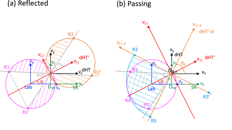
Figure 17. Diagrams to explain the maximum energy gain in shock drift acceleration. Panels (a) and (b) show reflected electrons and passing electrons, respectively. See the text in Appendix B for more details.
Download figure:
Standard image High-resolution image
Let us consider the maximum energy among the reflected electrons, measured in the SR frame. The energy in the SR frame can be measured based on the distance of the position in the velocity plane from the origin OSR. It is apparent that the position of R2 represents the farthest position among the reflected electrons (orange shaded regions) from OSR, even considering the 3D sphere of the distribution. This R2 is the intersection point between the orange circle and the upper gray line (the boundary of the loss cone). Let us obtain the coordinates of R1, R1', and R2. To make the argument simple in the dHT frame, we consider the coordinates parallel and perpendicular to the magnetic field, v∥, v⊥1, and v⊥2. See the red coordinates in the plot, denoted by dHT', where v⊥1 is in the vx
–vy
plane, while v⊥2 is perpendicular to this plane. In this coordinate system, the center of the magenta circle is located at  , while the center of the orange circle is located at
  . We first consider positions R1 and R1'. Let us use


where  and ϕ is the angle between the perpendicular velocity vector and the v⊥1 axis. The magenta sphere with its radius vm
, and the loss-cone boundary plane, where
and ϕ is the angle between the perpendicular velocity vector and the v⊥1 axis. The magenta sphere with its radius vm
, and the loss-cone boundary plane, where  (in the 2D plot, the solid gray lines), are given as

respectively. From the above Equations (B3) and (B4), the positions of R1 and R1' in the dHT' frame are obtained by using ϕ = 0 and ϕ = π, respectively, as


and


where
The reflection point R2 is the symmetric point of R1 with respect to the v⊥1 axis, given as


Let us calculate the energy of the reflected particle R2 in the SR frame, and the increase of the energy due to the reflection. In the dHT' frame, the origin OSR is located at  . Therefore, the maximum energy in the SR frame among the reflected electrons (the energy of R2) is given as
In the same way, we can obtain the energy at R1' before the reflection,  , by replacing v∥−R2 and v⊥1−R2 in Equation (B15) with
  and
and  , respectively. During the gyration before the reflection (i.e., gyration passing through R1 and R1'), position R1' is the place where the electron shows the minimum energy in the SR frame, because R1' is closest to OSR, which results in the maximum energy gain from R1' to R2. The energy increase from R1' to R2, represented by the increase of the Lorentz factor, Δγ, in the nonrelativistic limit is obtained as
The above equation gives the energy gain for the particle at R2, which shows the maximum energy among the reflected particles. However, this energy gain is not necessarily the maximum value of the energy gain among all of the reflected electrons. Let us obtain the energy gain for a general particle, whose pitch angle α ≥ α0. In Equation (B4), let us replace α0 with α, and use the velocity components before and after the reflection. Since we consider a general particle, we use a general angle ϕ in Equations (B1) and (B2), and let us denote the angles after and before the reflection as ϕa and ϕb , respectively. In the same way, in the following, the subscripts a and b in other quantities represent after and before the reflection, respectively. The energy in the SR frame after the reflection is obtained as
In the same way, the energy before the reflection is obtained using v∥−b
, v⊥1−b
, and v⊥2−b
. When v∥−b
= − v0, the parallel velocity reverses after the reflection, i.e., v∥−a
= v0. We also have a relation,  . Using these relations, the energy gain in the SR frame is calculated as
The energy gain is maximized when ϕa = 0 and ϕb = π. The above equation indicates that at a fixed angle α, the energy gain attains maximum when v0 reaches the largest value constrained by the conditions of Equations (B3) and (B4) before the reflection. In other words, the maximum energy gain is obtained at the surface of the magenta sphere. Substituting v∥ = v∥−b = − v0 and α0 = α in Equations (B3) and (B4), we obtain the following:
Substituting  from Equation (B19), ϕa
= 0, and ϕb
= π into Equation (B18), we obtain Δγ as a function of v0, as follows:
from Equation (B19), ϕa
= 0, and ϕb
= π into Equation (B18), we obtain Δγ as a function of v0, as follows:
This value takes the maximum value when the derivative dΔγ/dv0 becomes zero. The condition dΔγ/dv0 = 0 gives the parallel speed v0 as

and the maximum energy gain becomes

This maximum value should be obtained only when the angle α is larger than α0. From Equations (B19) and (B21), we obtain

When this value is larger than  , the derivative dΔγ/dv0 = 0 occurs in the region of α > α0. Therefore, Equation (B22) is valid only when
  calculated by Equation (B23) is larger than
  . Otherwise, dΔγ/dv0 = 0 occurs in the region α ≤ α0, and dΔγ/dv0 ≥ 0 in the region α ≥ α0, which means that Δγ is an increasing function of v0 in α ≥ α0. In this case, position R1 with the pitch angle α0 has the largest v0, and we should use Equation (B16) for Δγ.
Next, let us discuss passing electrons, which are particles within the loss cone. In Figure 17(b), we plot the mapping of the passing electrons (only half of the electrons with v⊥1 > 0 are shown). The gray shaded electrons within the loss cone (the sector bounded by OdHT
, R1, and R4) pass through the shock, and they are mapped into the region with light blue after passing to the downstream region. In the downstream region, the magnetic field By
increases, and as a result, the angle between the magnetic field vector and the x-axis changes from θ to  . Therefore, in plot (b), the new coordinates in the downstream region, v∥−d
-v⊥1−d
, are added as the orange arrows (denoted as dHT'-d frame). The electron denoted as R1, located at the crossing point between the gray line and the magenta circle, is mapped into R3, where the parallel velocity v∥−d
= 0. The loss-cone boundary line, R1-OdHT
is mapped into R3-OdHT
on the v⊥1−d
axis (orange line) in the dHT'-d frame. The position R3 is where the distance from OdHT
is the same as the distance between R1 and OdHT
. Position R4 represents the particle with the largest ∣v∥∣ (red line) in the dHT' frame, and the particles on the v∥ axis are mapped onto the v∥−d
axis (orange line), because v⊥1−d
= 0. R4 is mapped onto R5, where the distance from OdHT
is the same as the distance between R4 and OdHT
. Apparently, R3 is the farthest position from the origin in the SR frame, OSR. Therefore, among the passing electrons, the particle that has the maximum energy is R3 in the SR frame.
. Therefore, in plot (b), the new coordinates in the downstream region, v∥−d
-v⊥1−d
, are added as the orange arrows (denoted as dHT'-d frame). The electron denoted as R1, located at the crossing point between the gray line and the magenta circle, is mapped into R3, where the parallel velocity v∥−d
= 0. The loss-cone boundary line, R1-OdHT
is mapped into R3-OdHT
on the v⊥1−d
axis (orange line) in the dHT'-d frame. The position R3 is where the distance from OdHT
is the same as the distance between R1 and OdHT
. Position R4 represents the particle with the largest ∣v∥∣ (red line) in the dHT' frame, and the particles on the v∥ axis are mapped onto the v∥−d
axis (orange line), because v⊥1−d
= 0. R4 is mapped onto R5, where the distance from OdHT
is the same as the distance between R4 and OdHT
. Apparently, R3 is the farthest position from the origin in the SR frame, OSR. Therefore, among the passing electrons, the particle that has the maximum energy is R3 in the SR frame.
Since the distance OdHT -R3 is the same as the distance OdHT -R1, the coordinates at R3 in the dHT'-d frame are obtained as


In the dHT'-d frame, the position of OSR is given as  The energy of the particle at R3 in the SR frame (based on the distance between R3 and OSR) is obtained as
Note that in the upstream region, the particle at R1 is gyrating around the magnetic field, and this particle can appear at R1', the symmetric point of R1 with respect to the red line. In the downstream region, the particle at R3 is also gyrating around the magnetic field, and this particle can appear at R3'. Since R1' is the closest point to the origin OSR along the gyration of this particle in the upstream region, the energy gain becomes the largest for the particle that is mapped from R1' to R3.
The energy (Lorentz factor) increase, Δγ, between R1' and R3 is given as
Note that the largest energy gain for the passing electrons occurs only for the particles that are on the magenta spherical surface, not inside the sphere (we omit to show the proof, which can be done in the same way as the analysis of reflected electrons using Equation (B18), where we showed that the largest v0 gives the largest Δγ at a fixed α). Therefore, Equation (B27) shows the largest energy gain among all of the passing electrons. Comparing Equation (B16), Equation (B22), and Equation (B27), both the reflected electron and the passing electron show similar amounts of Δγ.
Let us evaluate Δγ using simulation parameters. We assume that θ = 25°, the ratio r( = Bd
/Bu
) = 4 (just as an example based on the simulation), which gives α0 = 45°, the shock speed vsh = 10.5vA0, and the maximum speed vm
= 40vA0 (based on a typical distribution in the shock transition region such as Figures 7(a) and 8(a)). Using these parameters and Equation (B11), we calculate Gθ
α0 = 6.38. In the simulation, we use vA0/c = 0.0177, and Equations (B22) and (B27) give Δγ = 0.137 and 0.084, respectively. Note that  based on Equation (B23) is 1.27, which is larger than
  . Therefore, we used Equation (B22) for the reflected electrons. Here we used θ = 25° as the value in the far-upstream region, but the angle between the magnetic field and the x-direction changes with time near the shock plane. In other words, the local shock angle changes with time, and it becomes a negative angle, such as −30° to −40° as in Figure 14(a). In a negative θ case, we can replace θ in Equations (B16), (B22), and (B27) with ∣θ∣. When we use r = 4, the angle
  , which is consistent with the angle in the downstream region in Figure 14(a). When ∣θ∣ = 30°, Gθ
α0 = 6.42, and
, which is consistent with the angle in the downstream region in Figure 14(a). When ∣θ∣ = 30°, Gθ
α0 = 6.42, and  in Equation (B23) is 1.08; therefore, we use Equation (B22) for reflected electrons. Equations (B22) and (B27) give Δγ = 0.175 and 0.107, respectively. Therefore, we conclude that Δγ ≲ 0.2 in shock drift acceleration, which is much smaller than Δγ observed in reconnection in the shock turbulence.