


Abstract
We have surveyed 21 reconnection exhaust events observed by Magnetospheric MultiScale in the low-plasma-β and high-Alfvén-speed regime of the Earth's magnetotail to investigate the scaling of electron bulk heating produced by reconnection. The ranges of inflow Alfvén speed and inflow electron βe covered by this study are 800–4000 km s−1 and 0.001–0.1, respectively, and the observed heating ranges from a few hundred electronvolts to several kiloelectronvolts. We find that the temperature change in the reconnection exhaust relative to the inflow, ΔTe, is correlated with the inflow Alfvén speed, VAx,in, based on the reconnecting magnetic field and the inflow plasma density. Furthermore, ΔTe is linearly proportional to the inflowing magnetic energy per particle,  , and the best fit to the data produces the empirical relation ΔTe = 0.020
  , i.e., the electron temperature increase is on average ∼2% of the inflowing magnetic energy per particle. This magnetotail study extends a previous magnetopause reconnection study by two orders of magnitude in both magnetic energy and electron β, to a regime that is comparable to the solar corona. The validity of the empirical relation over such a large combined magnetopause–magnetotail plasma parameter range of VA ∼ 10–4000 km s−1 and βe ∼ 0.001–10 suggests that one can predict the magnitude of the bulk electron heating by reconnection in a variety of contexts from the simple knowledge of a single parameter: the Alfvén speed of the ambient plasma.
Export citation and abstract BibTeX RIS

Original content from this work may be used under the terms of the Creative Commons Attribution 4.0 licence. Any further distribution of this work must maintain attribution to the author(s) and the title of the work, journal citation and DOI.
1. Introduction
Magnetic reconnection is a universal plasma process that is important in many astrophysical, solar, geophysical, and laboratory contexts. The process converts magnetic energy into plasma jetting and thermal and superthermal plasma energy. While plasma jetting is well established, both theoretically and observationally, the mechanism for particle heating in collisionless reconnection is still an area of active research. The aim of the present study is to investigate the controlling factors of electron bulk (∼thermal) heating in the high-Alfvén-speed, low-βe regime in Earth's magnetotail, a regime that is similar to that of the solar corona.
In situ observations of reconnection in near-Earth space have found that the degree of electron bulk heating in reconnection exhausts is vastly different in different regions. Generally, little (<5 eV) or no electron heating is detected in solar wind reconnection exhausts at 1 au (Gosling et al. 2007; Pulupa et al.2014) or even close to the Sun (Phan et al. 2021, 2022). At Earth's magnetopause, electron heating up to ∼40 eV is typically seen in the exhaust (e.g., Gosling et al. 1986; Phan et al. 2013). In contrast, electron bulk heating in the keV range is generally observed in reconnection exhausts in the magnetotail (e.g., Egedal et al. 2015; Wang et al. 2016; Ergun et al. 2018, 2020a, 2020b). These results suggest that the degree of electron heating depends on the plasma regime.
A statistical study of asymmetric magnetopause reconnection (Phan et al. 2013) reported evidence suggesting that electron bulk heating depends on the inflow Alfvén speed, which could help explain the different degrees of electron heating in different plasma parameter regimes. Specifically, the increase in the exhaust temperature relative to the inflow temperature was found empirically to be linearly proportional to the available inflow magnetic energy per proton–electron pair (or inflowing Poynting flux per particle density flux),  (=B2/μ0
N; Shay et al. 2014):
(=B2/μ0
N; Shay et al. 2014):

where mi is the proton mass, N is the inflow number density, B is the reconnecting magnetic field component, and VAL,asym is the hybrid inflow Alfvén speed, based on the reconnecting component of the magnetic field in the two inflow regions (Cassak & Shay 2007). The coefficient of 1.7% represents the empirical average percentage of available magnetic energy per particle that goes into the Te increase. A subsequent simulation scaling study using magnetopause-like parameter values also found the temperature increase to scale as  (Shay et al. 2014; Haggerty et al. 2015).
The magnetopause study (Phan et al. 2013) covered only a narrow range of parameter space: the observed maximum Alfvén speed was only 600 km s−1, βe was mostly >0.1, and the maximum electron temperature increase was only 70 eV. It is not clear whether relation (1) extends to higher-Alfvén-speed and low-βe plasma regimes. A case study using Cluster data in the low-βe magnetotail (Wang et al. 2016) found strong electron heating with a temperature increase up to 3.8 keV for an inflow VA of 2580 km s−1. That is, three times higher than predicted by the empirical relation (1). On the other hand, a recent theoretical study using kinetic Riemann simulations of guide field reconnection (Zhang et al. 2019) found that in the very-low-βe (<0.01) regime, the electron temperature increase does not scale linearly with the available magnetic energy per particle, but reaches a plateau instead. Zhang et al. (2019) found that in low-βe guide field reconnection, the released magnetic energy is split between bulk flow and ion heating, with little energy going to electrons.
In another theoretical study that addressed the universality of relation (1), Haggerty et al. (2015) found, through kinetic simulations, that it is the sum of the ion and electron temperature increase, not the electron temperature gain alone, that scales linearly with  . In terms of the heating mechanism, they found that electrons were energized as a result of multiple Fermi reflections due to electrons being trapped by large-scale field-aligned potentials in the exhaust (e.g., Egedal et al. 2008, 2015). Furthermore, Haggerty et al. (2015) found that a higher electron temperature in the inflow region led to larger exhaust potentials, which increased electron trapping and therefore electron heating, while lowering the ion heating by slowing the ions injected into the exhaust. This predicted competition between ion and electron heating has yet to be confirmed experimentally.
In this paper, we focus on the scaling of electron bulk heating in the low-βe and large-Alfvén-speed plasma regime by performing a comprehensive survey of reconnection events observed in the near-Earth magnetotail, where the range of βe is two orders of magnitude less than at the magnetopause, in a plasma parameter regime that could be applicable to the solar environment. Magnetotail reconnection typically involves nearly symmetric inflow conditions, and the guide magnetic field (normalized to the reconnecting field) is usually small (<0.2).
The electron temperatures used in the present study are obtained from the second moment of the distributions. Such temperatures are useful because they provide measures of the average energy in the electron rest frame. We shall refer to these temperatures as bulk temperatures and describe the increase in exhaust temperature (relative to the inflow temperature) as bulk heating.
Extending the scaling study to reconnection in the magnetotail is challenging because of the bursty nature of reconnection in this region, as well as the difficulties in measuring inflow plasma parameters accurately in the tenuous plasma environment. Furthermore, since the inflow conditions may evolve with time, it is not always straightforward to determine the inflow conditions that correspond to each outflow observation. Still, we were able to assemble a sufficient number of events to investigate the controlling factors of electron bulk heating in the high-Alfvén-speed, low-βe regime in Earth's magnetotail.
The paper is organized as follows. In Section 2, we describe the spacecraft instrumentation, and in Section 3, we present two case studies to illustrate the methodology. Section 4 describes the statistical study. The findings are summarized and discussed in Section 5.
2. Instrumentation
We use Magnetospheric MultiScale (MMS) Fast Survey mode data from the Earth's magnetotail between XGSM = −16.8 RE and XGSM = −27.5 RE. This study of large-scale heating in magnetotail reconnection exhausts does not require MMS high-resolution burst-mode data. We use magnetometer data at eight samples per second (Russell et al. 2016) and electron moment and distribution data from the Fast Plasma Investigation (FPI) at 4.5 s resolution (Pollock et al. 2016). We use proton density and velocity moments from the HPCA instrument at 10 s resolution (Young et al. 2016).
The HPCA instrument measures protons up to 40 keV (versus FPI, which has an upper energy limit of 30 keV) and therefore provides more accurate ion moments in the plasma sheet during active times when the ions are hot and the flow speeds are high. The HPCA instrument has a double coincidence system, which significantly reduces the background and improves the signal-to-noise ratio. It therefore provides reliable plasma (proton) density measurements, not only in the plasma sheet, but also in the low-density lobe.
The FPI instrument covers the energy range of the plasma sheet electron distribution well; thus, the plasma sheet electron temperature (i.e., the second moment of the electron distribution) is well measured by FPI. In the low-density lobe, on the other hand, the spacecraft potential is high, often making it challenging to accurately compute the moments of the electron distributions. The lobe electron temperature in this study is therefore obtained by Maxwellian fitting of the FPI electron distribution measurements averaged over the inflow interval. When fitting the lobe distributions, we exclude data points contaminated by photoelectrons at low energies and data points where the measurement uncertainty associated with the data point is near the detection limit (the one-count level) of the instrument (Oka et al. 2022).
The observations are presented in the Geocentric Solar Magnetospheric (GSM) coordinate system, with the origin at the center of the Earth, positive X pointing toward the Sun, with Y defined as the cross product of the GSM X-axis and the magnetic dipole axis and Z as the cross product of the X and Y axes. GSM is usually close to the coordinate system of the near-Earth magnetotail current sheet, with X being approximately along the reconnecting magnetic field (or outflow) direction, Z along the current sheet normal, and Y along the out-of-plane direction.
3. Examples of Magnetotail Reconnection Events
In this section, we present two individual magnetotail reconnection events observed by MMS to illustrate the methodology used in the statistical study.
3.1. Magnetotail Reconnection Event with Plasma Sheet Inflow
Figures 1(a)–(h) show MMS3 observations from 2017 July 17, 14:38–14:49 UT, when the spacecraft was located in the plasma sheet at XYZGSM = (−21.9, 6.8, 2.2)RE and encountered a high-speed tailward-to-earthward flow reversal. This event was previously reported by Oka et al. (2022). An interval of tailward-directed (negative VX ) high-speed flows was observed from 14:38:30 to 14:40:30 UT, followed by an interval of earthward (positive Vx ) high-speed flow at 14:45:30–14:49 UT (Figure 1(d)). Intervals in the tailward and earthward high-speed flow where the outflow velocity was relatively constant are marked with pairs of vertical red lines and discussed in more detail below. These observations of a tailward-to-earthward jet reversal with an associated predominantly negative to predominantly positive BZ reversal (the red curve in Figure 1(a)) are consistent with a reconnection X-line moving tailward past the spacecraft, resulting in an approximate spacecraft trajectory as indicated in Figure 1(i).
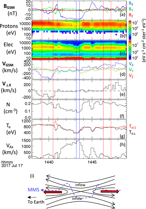
Figure 1. MMS3 observations of a magnetotail high-speed flow reversal event with plasma sheet inflow. (a) Magnetic field components in GSM coordinates. (b) Proton spectrogram in differential energy flux. (c) Electron spectrogram. (d) Proton velocity. (e) Proton VX component perpendicular to B. (f) Proton density. (g) Parallel (red) and perpendicular (black) electron temperature. (h) Alfvén speed based on proton density and BX . (i) Schematic of the reconnection geometry in the magnetotail and the approximate MMS spacecraft trajectory (the blue dashed curve). The pairs of red vertical lines in (a)–(h) mark outflow intervals and the pair of blue vertical lines mark an inflow interval.
Download figure:
Standard image High-resolution imageBetween the tailward and earthward jets, the spacecraft encountered a region of large ∣BX ∣ (the blue curve in Figure 1(a)), lower density (Figure 1(f)), and no perpendicular VX flow (Figure 1(e)), suggesting that the spacecraft encountered the reconnection inflow region during the passage of the X-line (Figure 1(i)).
To estimate the electron heating in the two (tailward and earthward) reconnection exhausts, we first selected appropriate outflow intervals. We are interested in direct heating in the fully developed exhaust, which is where the outflow jet has reached a quasi-steady level. Selecting an interval of quasi-steady outflow helps minimize the effects of changing inflow conditions. Thus, for each exhaust, we chose an interval of relatively stable outflow speed. Furthermore, to ensure a fair comparison between exhaust intervals from different events, we restricted the outflow observations to near the neutral sheet, by requiring the outflow velocity to have a significant component perpendicular to the magnetic field and a small ∣BX ∣ (<10 nT). The two selected intervals in the tailward and earthward exhausts are marked with pairs of red vertical lines. The average and standard deviation of the tailward and earthward exhaust electron temperatures were 928 ± 13 eV and 769 ± 15 eV, respectively.
Next, we identify an asymptotic (i.e., unmodified by reconnection) inflow interval that may correspond to the selected outflows. As mentioned above, the spacecraft likely encountered the inflow region between the tailward and earthward jets. The inflow interval should have large and stable ∣BX ∣, density lower than in the outflows, and no field-aligned electron temperature anisotropy. The latter condition is to avoid the inflow regions that have been modified by reconnection, such as field-aligned electron heating (e.g., Chen et al. 2008; Egedal et al. 2008; Shay et al. 2016). The interval between the two vertical blue lines in Figures 1(a)–(h) satisfies these criteria. The relatively high inflow density of 0.086 cm−3 (which was still lower than the outflow density of ∼0.2 cm−3, thus satisfying the conditions stated above) and electron temperature (∼415 eV) in this event indicate that the inflow was plasma sheet plasma, not lobe. Furthermore, the inflow interval had Te∣∣ ∼ Te⊥. The inflow Alfvén speed was 1488 km s−1, based on density ∼ 0.086 cm−3 and ∣BX ∣ ∼ 20 nT, and the inflow βe was 0.036.
The average electron temperature in the selected inflow interval was 415 eV (Figure 1(g)). Thus, the electron temperature increase, ΔTe = Te,outflow – Te,inflow, was 510 ± 13 eV for the earthward exhaust and 350 ± 15 eV for the tailward exhaust.
3.2. Magnetotail Reconnection Event with Lobe Inflow
A second example of a high-speed flow reversal event is shown in Figures 2(a)–(h). On 2019 August 8, at 13:54 UT, MMS was located in the magnetotail at XYZGSM = (−27.6, 0.5, 5.1)RE when it observed a high-speed VX flow reversal; a tailward (negative VX ) jet (13:54–14:00 UT) followed by an earthward (positive VX ) jet (14:15–14:27 UT; Figure 2(d)), with a correlated predominantly negative to predominantly positive BZ reversal (Figure 2(a), red curve), consistent with a reconnection X-line moving tailward past the spacecraft. Based on BX and VX time profiles, the effective spacecraft trajectory is shown in Figure 2(k) (blue dashed curve). Both the earthward and tailward flows contained intervals where VX had a component perpendicular to the magnetic field (Figure 2(e)) and ∣BX ∣ < 10 nT (Figure 2(a)), implying that the spacecraft observed the jets in the vicinity of the neutral sheet, away from the plasma sheet boundary layer (PSBL) during those times. Electron temperatures of 500–600 eV were observed in the tailward jet, while the electron temperature in the earthward jet was higher, at 1–3 keV (Figure 2(g)).

Figure 2. MMS3 observations of a magnetotail high-speed flow reversal event with lobe inflow. (a) Magnetic field. (b) Proton spectrogram. (c) Electron spectrogram. (d) Proton velocity. (e) Proton VX component perpendicular to B. (f) Proton density. (g) Parallel (red) and perpendicular (black) electron temperature. (h) Alfvén speed based on proton density and BX . (i) and (j) Maxwellian fit (red curve) to the average electron distribution function measurements in the two lobe (inflow) intervals marked by pairs of blue vertical lines in (a)–(h). Only the red data points have been used for the Maxwellian fitting (see the text for details). The two Maxwellian fits in (i) and (j) result in inflow electron temperatures of 89 eV and 83 eV, respectively. The solid black curve in (j) and (k) is the one-count level for the electron instrument. The measurement uncertainty for each data point is displayed with black vertical lines. (k) Schematic of the reconnection geometry in the magnetotail and approximate spacecraft trajectory (blue dashed curve).
Download figure:
Standard image High-resolution imageAs with the previous example (Section 3.1), to evaluate the electron heating we selected exhaust intervals where the ion outflow velocity had reached a stable level, had a significant VX component perpendicular to the magnetic field, and small ∣BX ∣. The selected outflow intervals are marked with red vertical lines in Figures 2(a)–(h) in both the tailward and earthward exhaust.
The average electron temperature in the selected tailward exhaust interval was 521 ± 13 eV. To estimate the heating in this exhaust, we compare with the closest inflow interval. Between the tailward and earthward jet (∼14:00–14:15 UT), the spacecraft entered a region of large BX values (mostly >10 nT), consistent with the spacecraft being in the vicinity of the inflow region (Figure 2(k)). The density and temperature in this interval varied, and earthward-directed (positive Vx ) field-aligned flows were observed intermittently, indicating that the spacecraft intermittently encountered the outer edge of the exhaust in the PSBL. However, there were two brief intervals (between pairs of vertical blue lines) within this large-BX region where the peak electron energy flux was below ∼200 eV and density <0.05 cm−3, and with no earthward flows, indicating encounters with the cold magnetotail lobe.
One of the lobe intervals was observed adjacent to the tailward exhaust, and we use this interval to estimate the upstream conditions for the tailward exhaust interval. Level 2 electron moments are not available, due to large photoelectron effects in this cold and tenuous lobe. We therefore obtained the inflow electron temperature by fitting the average omnidirectional electron distribution measurements with a Maxwellian distribution, as shown in Figure 2(i). When fitting the distributions, we excluded data points contaminated by photoelectrons at low energies and data points at high energies where the error bars extend below the detection limit (the one-count level) of the instrument (Oka et al. 2022). The best-fit Maxwellian distribution corresponds to an electron temperature of 89 eV, which we used as an estimate for the inflow temperature, in lieu of electron moments. From this, we found the electron temperature increase in the tailward exhaust interval to be 432 ± 13 eV. The inflow Alfvén speed in this lobe interval was 2285 km s−1, with 0.033 cm−3 inflow density and BX = 18.9 nT. Inflow βe was 0.0033.
The average electron temperature for the earthward exhaust interval was 1390 ± 272 eV. We avoid the PSBL interval, as discussed above, and use the second lobe encounter at ∼14:06:30–14:07:00 UT (marked by the vertical blue lines in Figures 2(a)–(h)) to estimate the upstream conditions for the earthward exhaust. Again, we estimate the electron temperature in this lobe interval by Maxwellian fitting (Figure 2(j)) and obtain a lobe inflow temperature of 83 eV. Thus, the estimated electron temperature increase was 1307 eV ± 272 for the earthward flow interval. For this lobe interval, the inflow Alfvén speed was 2128 km s−1, the inflow density was 0.031 cm−3, BX = 17.3 nT, and βe was 0.0035.
4. Statistical Study
Using the methodology illustrated in the two case studies (Section 3), we examined the electron temperature change from inflow to outflow (ΔTe) for 21 magnetotail reconnection exhausts in the data set described below (Section 4.1) and studied how ΔTe depends on plasma and field conditions in the inflow region.
4.1. MMS Data Set of Magnetotail High-speed Flow Reversal Events and Selection Criteria
The goal of the present study is to investigate direct heating by reconnection in the fully developed exhausts, not by secondary heating processes farther downstream of the X-line, e.g., in the flow-breaking region (e.g., Runov et al. 2011). To ensure that we are observing the exhaust away from the flow-breaking region, we restricted the data set to plasma jet reversals, like those presented above in Section 3. Such events are generally associated with the passage of a reconnection X-line, so that the observations are away from the flow-breaking region, which is located far downstream.
The events were identified based on the presence of tailward-to-earthward fast plasma sheet ion flow reversals with correlated negative to positive BZ reversals. These signatures indicate the tailward retreat of a reconnecting X-line, which is a typical behavior of magnetotail X-lines (Hones 1979). The jet reversal events were identified using 4 yr of MMS3 magnetotail observations from 2017 to 2020. We found 74 events that satisfied these initial criteria. We then imposed several additional selection criteria to ensure that the selected outflow and inflow intervals were appropriate for the heating study.
For the outflow intervals, we required the following:
- 1.The interval should be relatively close to the flow reversal to avoid effects from additional heating processes farther downstream.
- 2.The interval should have a relatively stable outflow speed, to be in the fully developed exhaust and to avoid sampling the diffusion region.
- 3.The interval should have a significant VX component perpendicular to the magnetic field and ∣BX ∣ < 10 nT. This ensures that the observations are obtained relatively close to the current sheet midplane for fair comparisons between exhaust intervals from different events.
For the inflow intervals, we required the following:
- 1.The interval should be observed as close to the selected exhaust interval as possible, but should not contain any parts of the exhaust itself.
- 2.The interval should have a large and stable ∣BX ∣ > 10 nT.
- 3.The density should be less than the exhaust density.
- 4.
In some cases, the inflow was not observed, it was observed too far from the outflow, or two or more candidate inflow intervals with different plasma properties were observed near the outflow and we could not determine which one corresponded to the selected outflow interval. Such events were not included.
After applying these criteria, we were left with 14 high-speed flow reversals where at least one, and often both, of the bidirectional jets and their associated inflows satisfied the selection criteria. This resulted in a total of 21 exhaust events, where 10 of the exhausts were directed tailward and 11 earthward. Most (18 of 21) inflow observations, including the two examples shown above (Section 3), were obtained when the spacecraft entered the inflow region between the tailward and the earthward jets. The 21 events are listed in Table 1.
Table 1. List of Events
| Event | Inflow Interval | Exhaust Interval | ∣Bx,in∣(nT) | Nin(cm−3) | VAx,in(km s−1) | βe,in | Nout(cm−3) | Te,in(eV) | Te,out(eV) | ΔTe(eV) |
|---|---|---|---|---|---|---|---|---|---|---|
| 1 | 2017-07-11/22:31:10–2017-07-11/22:32:00 | 2017-07-11/22:32:15–2017-07-11/22:33:15 | 11.6 | 0.051 | 1125 | 0.12 | 0.062 | 826 | 1045 | 219 |
| 2 | 2017-07-11/22:38:47–2017-07-11/22:39:01 | 2017-07-11/22:36:59–2017-07-11/22:37:43 | 15.1 | 0.040 | 1641 | 0.070 | 0.151 | 1003 | 1385 | 382 |
| 3 | 2017-07-17/07:50:25–2017-07-17/07:50:44 | 2017-07-17/07:48:02–2017-07-17/07:49:12 | 20.2 | 0.051 | 1931 | 0.080 | 0.066 | 1584 | 2280 | 696 |
| 4 | 2017-07-17/14:43:11–2017-07-17/14:43:32 | 2017-07-17/14:39:12–2017-07-17/14:40:29 | 20.0 | 0.086 | 1488 | 0.036 | 0.204 | 415 | 928 | 513 |
| 5 | 2017-07-17/14:43:11–2017-07-17/14:43:32 | 2017-07-17/14:46:18–2017-07-17/14:47:11 | 20.0 | 0.086 | 1488 | 0.036 | 0.207 | 415 | 769 | 354 |
| 6 | 2017-07-26/00:13:03–2017-07-26/00:13:32 | 2017-07-26/00:18:04–2017-07-26/00:18:24 | 21.9 | 0.018 | 3909 | 0.0012 | 0.043 | 82 | 3377 | 3295 |
| 7 | 2017-07-26/13:00:16–2017-07-26/13:02:00 | 2017-07-26/13:05:22–2017-07-26/13:06:58 | 14.9 | 0.077 | 1172 | 0.23 | 0.082 | 1678 | 2042 | 364 |
| 8 | 2017-08-23/14:44:12–2017-08-23/14:45:06 | 2017-08-23/14:49:59–2017-08-23/14:50:40 | 25.6 | 0.042 | 2728 | 0.0016 | 0.141 | 63 | 1976 | 1913 |
| 9 | 2017-08-23/15:22:32–2017-08-23/15:23:30 | 2017-08-23/15:29:38–2017-08-23/15:33:00 | 28.1 | 0.058 | 2622 | 0.0019 | 0.212 | 64 | 1595 | 1530 |
| 10 | 2017-08-24/06:33:16–2017-08-24/06:33:54 | 2017-08-24/06:31:48–2017-08-24/06:32:26 | 24.3 | 0.16 | 1322 | 0.16 | 0.215 | 1441 | 1749 | 308 |
| 11 | 2018-08-18/07:35:30–2018-08-18/07:36:27 | 2018-08-18/07:38:14–2018-08-18/07:39:18 | 20.9 | 0.035 | 2493 | 0.0033 | 0.219 | 102 | 1454 | 1352 |
| 12 | 2018-09-10/23:43:10–2018-09-10/23:43:42 | 2018-09-10/23:39:14–2018-09-10/23:39:44 | 32.3 | 0.23 | 1482 | 0.076 | 0.598 | 870 | 1167 | 297 |
| 13 | 2018-09-10/23:58:38–2018-09-10/23:59:02 | 2018-09-10/23:59:42–2018-09-11/00:01:24 | 26.1 | 0.32 | 1009 | 0.13 | 0.508 | 705 | 911 | 206 |
| 14 | 2019-08-05/15:54:16–2019-08-05/15:56:04 | 2019-08-05/15:52:08–2019-08-05/15:52:50 | 30.7 | 0.27 | 1290 | 0.052 | 0.570 | 452 | 856 | 404 |
| 15 | 2019-08-05/16:17:42–2019-08-05/16:18:00 | 2019-08-05/16:19:25–2019-08-05/16:21:22 | 24.7 | 0.042 | 2691 | 0.011 | 0.222 | 413 | 2029 | 1616 |
| 16 | 2019-08-08/14:01:37–2019-08-08/14:01:51 | 2019-08-08/13:57:50–2019-08-08/13:58:41 | 18.9 | 0.033 | 2285 | 0.0033 | 0.393 | 89 | 521 | 432 |
| 17 | 2019-08-08/14:06:24–2019-08-08/14:06:52 | 2019-08-08/14:15:48–2019-08-08/14:16:32 | 17.3 | 0.031 | 2128 | 0.0035 | 0.224 | 83 | 1390 | 1307 |
| 18 | 2019-08-12/14:21:26–2019-08-12/14:22:02 | 2019-08-12/14:19:54–2019-08-12/14:21:04 | 16.1 | 0.18 | 834 | 0.13 | 0.483 | 472 | 660 | 188 |
| 19 | 2019-08-12/14:21:26–2019-08-12/14:22:02 | 2019-08-12/14:26:44–2019-08-12/14:27:48 | 16.1 | 0.18 | 834 | 0.13 | 0.513 | 472 | 593 | 121 |
| 20 | 2019-09-08/16:21:42–2019-09-08/16:22:18 | 2019-09-08/16:17:24–2019-09-08/16:18:00 | 16.5 | 0.017 | 2773 | 0.0041 | 0.094 | 162 | 1669 | 1506 |
| 21 | 2019-09-09/02:25:19–2019-09-09/02:25:44 | 2019-09-09/02:35:32–2019-09-09/02:36:40 | 17.2 | 0.010 | 3692 | 0.0047 | 0.108 | 337 | 2849 | 2512 |
Note. Events 1 and 2 were reported by Torbert et al. (2018). Event 3 was reported by Rogers et al. (2019). Events 4 and 5 were reported by Oka et al. (2022).
Download table as: ASCIITypeset image
In the magnetotail, spacecraft typically pass through a reconnection event in an along-the-current sheet trajectory (as opposed to across the current sheet at the magnetopause). Combined with the dynamic nature of tail reconnection, this can make it challenging to deduce which inflow and outflow intervals are associated with each other. Even with the strict selection criteria, which left us with only 21 events, we cannot be 100% certain that every selected outflow is associated with the selected inflow or that the inflow did not change during the time between the two observations. These uncertainties are discussed in more detail below, in Section 4.4. The selected events (Table 1) thus constitute our best attempt to pair up inflow and outflow intervals.
Some of the events have been reported previously. For example, the exhausts in events 1 and 2 (Table 1) are from the flow reversal associated with the electron diffusion region encounter reported by Torbert et al. (2018). As mentioned above, we are interested in the fully developed reconnection jet downstream of the X-line in this study, and we do not include observations inside the diffusion region, which was the focus of the Torbert et al. (2018) study. The well-studied tail reconnection event of 2017 July 26 (Ergun et al. 2018, 2020a, 2020b) could not be included in our study because we were unable to identify an unperturbed inflow interval.
In near-Earth magnetotail reconnection, the guide field is typically small (<0.2), and the inflow is generally symmetric on the two sides of the magnetotail current sheet. Thus, the reconnection geometry in the events presented here is different from the magnetopause reconnection exhausts studied by Phan et al. (2013), where the inflow was asymmetric and the guide field varied between zero and one.
4.2. Statistical Findings of Electron Bulk Heating Dependence on Inflow Parameters
Figure 3(a) shows the electron temperature change from inflow to outflow, ΔTe, versus the inflow Alfvén speed based on the XGSM (roughly the reconnecting) component of the magnetic field (VAx,in) for the 21 magnetotail reconnection exhausts in the data set described above (Section 4.1; see also Table 1). Events with lobe inflow are marked in blue and are generally characterized by low inflow density (Figure 3(c)) and low inflow electron temperature (Figure 3(e)). Events with plasma sheet inflow are in black and are characterized by higher inflow electron temperatures. ΔTe is well correlated with VAx,in, but the dependence is not linear. To deduce the power of the VAx,in dependence, we fitted the data to the function ΔTe = constant ∗  . The best fit (the black dashed curve in Figure 3(a)) gives the relation ΔTe = 1.77 × 10⁻⁴
 , indicating that ΔTe scales with
  . Refitting the data to
  gives ΔTe = 2.06 × 10⁻⁴
 (the red dashed curve in Figure 3(a)), where ΔTe and VAx,in are in units of eV and km s−1, respectively.
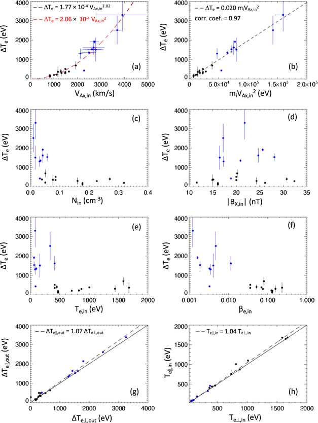
Figure 3. Electron temperature change ΔTe vs. inflow parameters. Events with lobe inflow are in blue and events with plasma sheet inflow are in black. (a) ΔTe vs. inflow Alfvén speed based on the reconnecting field component BX . (b) ΔTe vs. available magnetic energy per particle. (c) ΔTe vs. inflow density. (d) ΔTe vs. inflow ∣BX ∣. (e) ΔTe vs. inflow electron temperature. (f) ΔTe vs. inflow electron β. (g) Outflow ΔTe∣∣ vs. outflow ΔTe⊥. (h) Inflow Te∣∣ vs. inflow Te⊥. The black solid lines in (g) and (h) mark Te∣∣ = Te⊥, while the dashed lines in (b), (g), and (h) are linear least-squares fits to the data.
Download figure:
Standard image High-resolution imageSince  represents the available magnetic energy per particle from both sides of the current sheet, the dependence on
  means that there is a linear dependence between the available magnetic energy per particle and the temperature increase (Figure 3(b)). Linear fitting of the data gives the empirical relation:

This relation is remarkably similar to the relation obtained using magnetopause observations, ΔTe = 0.017 mi
 (Phan et al. 2013), which was for a much lower magnetic energy per particle regime and for highly asymmetric reconnection. The empirical relation in (2) implies that the electron temperature increase is ∼2% of the available magnetic energy per particle. In terms of energy partition, for the simplified case of isotropic plasmas, the percentage of the inflowing Poynting flux per particle density flux converted into electron enthalpy flux is given by [γ/(γ − 1)]ΔTe/mi
 = 0.020 γ/(γ − 1) = 5%, where γ = 5/3 is the ratio of the specific heats.
We also performed linear least-squares fitting for the 12 data points with plasma sheet inflow and the nine events with lobe inflow separately. The linear fit for the plasma sheet events (black dots) gives the relation ΔTe = 0.018 mi
 , while for the lobe events (blue dots), one obtains ΔTe = 0.020
  . Thus, the scalings of the two separate groups of events are essentially the same as the combined result.
We have also examined how ΔTe might depend on the individual inflow parameters Bx,in, Nin, and Te,in. No discernible relationship is seen between ΔTe and Bx,in (approximately the reconnecting field) in this data set (Figure 3(d)). However, the range of ∣Bx,in∣ values in this data set (∼15 nT to ∼30 nT) could be too small to reveal any dependency. The inflow density, on the other hand, covers more than one order of magnitude (Figure 3(c)) and shows an inverse relationship with the temperature increase: events with large electron temperature increases (say >1 keV) have inflow density <0.06 cm−3. This correlation is understandable, since a lower inflow density means more magnetic energy per particle is available to heat the particles.
Figure 3(e) shows the electron temperature change versus inflow electron temperature. The highest heating events are seen at low inflow electron temperatures. However, this apparent relationship should be viewed with care, since the high heating events correspond to the inflows being in the low-density lobe (marked in blue), where the inflow electron temperature tends to be low.
In terms of the dependence on inflow βe, Figure 3(f) shows that there is an inverse relation between inflow βe and ΔTe.
We have also investigated the parallel and perpendicular electron temperature changes separately. Figure 3(g) shows that the parallel heating was slightly more than the perpendicular heating, with ΔTe∣∣,out = 1.07 ΔTe⊥,out (the dashed line in Figure 3(g)). The near-isotropic electron heating for this low-guide-field magnetotail data set is in agreement with previous studies showing low heating anisotropy for low-guide-field cases (Chen et al. 2008; Phan et al. 2013; Li et al. 2018).
When selecting inflow intervals, one criterion was isotropic inflow electron temperature, to avoid sampling any part of the inflow that has been modified (preheated) by reconnection (Chen et al. 2008; Egedal et al. 2008). Figure 3(h) confirms that Te∣∣ ∼ Te⊥ for all inflow intervals.
4.3. Electron Heating Normalized to Inflow Parameters
We examined (in Figure 4(a)) whether the percentage of heating relative to the available magnetic energy per particle is dependent on the inflow electron temperature and found no clear dependence. The data in Figure 4(a) also provide an alternative way to infer the coefficient in relation (2). The average and standard deviation of ΔTe/mi
 are 0.019 ± 0.005. The standard deviation of 0.005 suggests that relation (2) is statistically the same as the magnetopause expression in relation (1).

Figure 4. Electron temperature change normalized to inflow parameters. Events with lobe inflow are in blue and events with plasma sheet inflow are in black. (a) ΔTe normalized to mi
 vs. inflow electron temperature. (b) ΔTe and available magnetic energy per particle normalized to the inflow electron temperature. (c) ΔTe normalized to the inflow electron temperature vs. the inflow electron β. (d) ΔTe vs. the exhaust density divided by inflow density. The dashed line in (b) is the linear least-squares fit to the data.
Download figure:
Standard image High-resolution image
Figure 4(b) shows electron heating versus available magnetic energy per particle with both parameters normalized to the inflow temperature Te,in. The linear fit (dashed curve) to the normalized data is excellent, with ΔTe/Te,in = 0.021  /Te,in, i.e., nearly identical to the relation for the unnormalized values (Figure 3(b)). While the similarity between the normalized and unnormalized empirical relations is somewhat trivial, the positions of the data points are reordered in Figure 4(a) due to the normalization to the individual inflow Te for each event.
There is also a linear dependence between ΔTe/Te,in and the inflow βe, with ΔTe/Te,in inversely proportional to βe (Figure 4(c)). This relation is equivalent to the relation in Figure 4(a) (with a factor of a half difference) since  /2Te,in.
Figure 4(d) shows electron heating versus the ratio of exhaust (outflow) density to inflow density. Interestingly, six of the lobe inflow events have a density ratio larger than 4. A density increase from inflow to exhaust by more than a factor of 4 is not expected of density compression across traditional switchoff slow shocks at the exhaust boundaries (Lin & Lee 1993). While we cannot entirely exclude the possibility that the large density ratios could be a side effect of mismatched inflow and outflow intervals (see Sections 4.1 and 4.4), another possible explanation is that the large density ratios are a consequence of additional density compression occurring in the low-β magnetotail exhaust. For example, it has been well established that when magnetic islands develop during reconnection, significant compression of the density takes place, leading to higher outflow densities (Drake et al. 2006; Li et al. 2018).
4.4. Sources of Uncertainty
The error bars in Figure 3 represent the standard deviations for the data in the observed intervals. These error bars should be interpreted with caution, since there are additional uncertainties that cannot be quantified.
One important source of uncertainty arises from the fact that the outflow and the inflow are not observed simultaneously, but with a delay of 1–9 minutes (Table 1). In our analysis, we have assumed that the inflow conditions remained stable for this length of time; however, this stability cannot be checked. To minimize this uncertainty, we selected only intervals where the outflow speed is stable for several minutes.
Another source of uncertainty is the choice of inflow interval. In some events, two or more candidate inflow intervals were observed near the outflow. For consistency, we chose the inflow interval observed closest to the selected outflow interval.
5. Discussion and Summary
We have performed a survey of electron heating in symmetric reconnection in the high-Alfvén-speed and low-βe regime of Earth's magnetotail, in a plasma regime that is comparable to the solar corona. The magnetotail study extends a previous asymmetric magnetopause reconnection study by two orders of magnitude in both magnetic energy and βe. Remarkably, the scaling of the magnetotail reconnection electron heating is similar to that of the magnetopause.
The present study has found that the electron bulk heating is linearly proportional to the available magnetic energy per particle (or Poynting flux per inflowing particle density flux),  , with an empirical relation of ΔTe = 0.020
  . For the simplified case of isotropic plasmas, the percentage of the inflowing Poynting flux per inflowing particle density flux converted into electron enthalpy flux is given by [γ/(γ − 1)]ΔTe/
 = 0.02 γ/(γ − 1) = 5%, where γ = 5/3 is the ratio of the specific heats. Our results indicate that there is a linear dependence of the bulk electron heating on the inflowing magnetic energy per particle, extending from VA = 800 km s−1 to 4000 km s−1 and βe from 0.001 to 0.1. Combined with earlier magnetopause results in the high-βe regime (Phan et al. 2013), which found the empirical relation of ΔTe = 0.017
  , for VA = 10–600 km s−1 and βe = 0.1–10, the linear dependence of the bulk electron heating on the inflowing magnetic energy per particle appears to be valid for VA = 10–4000 km s−1 and βe = 0.001–10.
While the scaling study at the magnetopause covered the range of guide field from zero to one, the magnetotail study addresses only low-guide-field (typically <0.2) reconnection, due to the geometry of the reconnecting current sheet in this region. Thus, whether electron heating levels off at low βe in guide field reconnection, as predicted by Zhang et al. (2019), is unexplored. Nevertheless, our study suggests that linear scaling for electron heating in reconnection exhausts exists over a large plasma parameter range, at least for low guide fields.
In the magnetotail, it is well known that there is often a transition from plasma sheet (low inflow Alfvén speed) reconnection to lobe (high inflow Alfvén speed) reconnection during a reconnection event (e.g., Hones 1979; Baker et al. 2002; Cao et al. 2008; Oka et al. 2022). Relation (2) could account for the observed large increase of exhaust electron temperature during that transition.
The highest VA and lowest βe included in the present study may have applications to solar and astrophysical contexts. For example, in the solar corona, with an ambient magnetic field of ∼100 Gauss and plasma number density ∼1010 cm−3, the Alfvén speed would be ∼2200 km s−1, and the empirical relation (2) predicts reconnection electron heating of ∼1 keV (or ∼107 K).
A practical implication of the empirical scaling relations (1) and (2) is that the amount of electron heating is predictable without detailed knowledge of the heating mechanism or mechanisms. The validity of the relation  over such an extended range of VA and βe suggests that either the heating mechanism is the same over that range or that the detailed mechanism does not matter when it comes to the partition of energy. This is intriguing, since high-electron-exhaust-temperature events in the tail tend to be associated with highly turbulent exhausts with large and spiky parallel electric fields (e.g., Ergun et al. 2018, 2020a, 2020b), while the exhausts in low-temperature events are characteristically laminar (e.g., Torbert et al. 2018). Different heating mechanisms have been proposed for these contrasting regimes. Ergun et al. (2018) proposed that large-amplitude and bursty parallel electric fields could account for the heating and acceleration of electrons in the low-density (i.e., low-βe and high-Alfvén-speed) regime. In contrast, in a simulation study of laminar exhausts, Haggerty et al. (2015) found that the electron heating is a result of Fermi acceleration, with electrons going through multiple reflections due to the presence of large-scale field-aligned trapping potentials in the exhaust. The lower the βe, the larger the trapping potential and hence electron heating (Egedal et al. 2015).
Regardless of the detailed heating mechanisms, the magnetotail and magnetopause (Phan et al. 2013) studies together suggest that, at least for small guide fields, there is a linear relation between the available magnetic energy per particle and reconnection electron heating, ΔTe ∼ 0.020  , for VA ranging from 10 to 4000 km s−1 and βe = 0.001–10. The validity of relation (2) over such a large plasma parameter range suggests that one can predict the magnitude of the bulk electron heating by reconnection in a variety of contexts from the simple knowledge of a single parameter: the Alfvén speed of the ambient plasma.
Acknowledgments
This research was supported by NASA grants 80NSSC18K1380, 80NSSC20K1781, 80NSSC20K0627, 80HQTR21T0103, and NASA contract NNG04EB99C (at SWRI).