

Abstract
Energy, water, and agricultural resources across the globe are highly interconnected. This interconnectivity poses science challenges, such as understanding and modeling interconnections, as well as practical challenges, such as efficiently managing interdependent resource systems. Using the US as an example, this study seeks to define and explore how interconnectivity evolves over space and time under a range of influences. Concepts from graph theory and input–output analysis are used to visualize and quantify key intersectoral linkages using two new indices: the 'Interconnectivity Magnitude Index' and the 'Interconnectivity Spread Index'. Using the Global Change Analysis Model (GCAM-USA), we explore the future evolution of these indices under four scenarios that explore a range of forces, including socioeconomic and technological change. Analysis is conducted at both national and state level spatial scales from 2015 to 2100. Results from a Reference scenario show that resource interconnectivity in the US is primarily driven by water use amongst different sectors, while changes in interconnectivity are driven by a decoupling of the water and electricity systems, as power plants become more water-efficient over time. High population and GDP growth results in relatively more decoupling of sectors, as a larger share of water and energy is used outside of interconnected sector feedback loops. Lower socioeconomic growth results in the opposite trend. Transitioning to a low-carbon economy increases interconnectivity because of the expansion of purpose-grown biomass, which strengthens the connections between water and energy. The results highlight that while some regions may experience similar sectoral stress projections, the composition of the intersectoral connectivity leading to that sectoral stress may call for distinctly different multi-sector co-management strategies. The methodology we introduce here can be applied in diverse geographical and sectoral contexts to enable better understanding of where, when, and how coupling or decoupling between sectors could evolve and be better managed.
Export citation and abstract BibTeX RIS
1. Introduction
Energy, water, and land resources across the globe are both strained and highly interconnected [1–4]. The scarcity and interdependency of energy, water, and land resources is well documented and can result in both synergies and trade-offs among sectors [5–23]. The strength of these interconnections determines the downstream impacts of shortages in one resource on the others. The water sector provides illustrative examples of the implications of resources constraints and sectoral interconnectivity. Globally, almost four billion people already experience severe water scarcity in at least one month per year [2, 24, 25]. In the US, half of river basins may be unable to meet monthly water demands by 2070 [26]. Urbanization and increasing consumption patterns are shifting the dynamics of these interconnections, which vary across the world. While globally agriculture remains the dominant user of water [27], in the US 40% of all water withdrawn is now being used for cooling power plants to generate electricity [28, 29]. This leaves the hydroelectric grid vulnerable to worsening hydrometeorological conditions such as droughts [30–33]. Increasing demands for energy has led to an expansion of biofuels in many regions, resulting in competition with food crops for land, nutrient, and water resources [34–36], as well as competition with the power and municipal sectors for water resources. To manage freshwater scarcity, alternate water sources (such as desalination, ground-water pumping, and water transfers) are increasingly being accessed, but they carry significant energy consumption requirements [16, 30, 37, 38]. These are just a few (of many) examples of strained resources and their interconnections, focusing on water-driven interconnections as an example.
Forces such as population growth, technological change, urbanization, increasing consumption, and climate change are poised to not only worsen existing resource constraints, but also to accelerate the integration of resource systems [9, 18, 19, 39–42]. As these systems become more integrated, resource constraints in any given sector have the potential to propagate across multiple sectors in nonlinear and unexpected ways [6]. Institutions that are responsible for crafting policies, plans, and strategies in the energy, water, and land sectors are typically competing for scarce institutional and financial resources to meet their sectoral goals. As opposed to single-sector planning, strategic multi-sector planning that seeks out synergies [14], and avoids conflicts [43], is more likely to receive support because it promotes efficiency and resilience. The nature of cross-sectoral opportunities and threats in any particular region will depend on the degree of sectoral interconnectivity that exists, which can vary depending on the spatial and temporal scale being considered [30, 40, 44–49].
Several reviews of past intersectoral analysis methodologies [41, 50–56] show that existing studies on the subject generally analyze intersectoral linkages in two main ways: (a) by examining indirect impacts as a result of the interconnections between a chosen subset of possible linkages [11, 16, 48, 49, 57–60]; or (b) by simultaneously analyzing multiple single-sector indices [8, 61–64]. The list below summarizes some of the key examples from this literature.
(a) Indirect impacts cited include:
- Increased emissions and water demands in response to increasing livestock productivity and crop yields [11];
- increased global costs and energy consumption to meet water and climate Sustainability Development Goals [16];
- export of scarce water, energy and land resources embodied in traded products both regionally and internationally leading to environmental degradation [23, 48, 49];
- global efforts to simultaneously reduce projected increases in food (60%), energy (60%) and water (20%) consumption from 2015 to 2050 [58];
- implications of water treatment and environmental flow constraints on energy and land use [59, 60];
(b) Combinations of various sectoral indices have been used in different studies to capture multi-sector interactions, including:
- A normalized index to capture the mass and economic value of water and energy embodied in agricultural products in a region [8];
- a combination of 14 different indicators across water, energy, and land (including resource availability, access, pollution, droughts, heat exposure) to capture global exposure of vulnerable populations to multi-sector hotspots [61];
- a combination of food, energy, and water sub-indices, which capture access and availability of resources to rank and assess multi-sector sustainability, either globally or for individual countries or regions (e.g. river basins) [8, 62, 63].
These past studies, looking at indirect impacts of interconnectivity and combined sector-specific indices, identify some of the key sectoral linkages and show that the interconnections between various sectors lead to important indirect impacts. No previous study, however, has focused exclusively on quantifying the degree of intersectoral connectivity and how it may evolve into the future under various scenarios.
In this paper, we complement these past studies by focusing explicitly on identifying and analyzing the 'degree of interconnectivity' amongst sectors as opposed to the indirect impacts which are a result of the interconnectivity. We define interconnectivity here to mean the strength, number, and spread of linkages between different systems. To capture these characteristics, we use the concept of 'network density' from graph theory (used previously in social and governance network studies) [65–68], as well as an inverse root mean square error (RMSE) measure [69], to establish two interconnectivity indices: the 'Interconnectivity Magnitude Index' (Magnitude) and the 'Interconnectivity Spread Index' (Spread). Both indices are defined in detail in the Methodology section. As pressures on scarce resources increase, it will become increasingly important to better understand the nature of interconnections between different systems. In this study, using the Magnitude and Spread indices, we seek to help with this understanding and answer the following research questions:
- (a)How will interconnectivity between the energy, water and agriculture sectors evolve across space and time in the United States?
- (b)How will this evolution of interconnectivity vary in response to socio-economic and technological change?
The remainder of this paper is organized as follows. Section 2 describes the novel methodology used to measure interconnectivity. Section 3 presents model outputs together with an analysis of the results. Section 4 is a discussion of the results and how they relate to other studies. Finally, Section 5 provides a summary of the paper, addresses the study's limitations, and describes potential future extensions of the study.
2. Methodology
In this paper, we define two new interconnectivity indices that capture the strength and spread of intersectoral connections in chosen sectors in a region. More specifically, the 'Interconnectivity Magnitude Index' (Magnitude) is used to quantify the share of physical commodities in each sector flowing to other sectors that are part of feedback loops (i.e. when sectors are mutually connected by both inputs and outputs from each). Sectors that are part of feedback loops are classified as 'feedback sectors', while 'unidirectional sectors' are defined as those that have only unidirectional connections with other sectors and are thus not part of any feedback loops. The 'Interconnectivity Spread Index' (Spread) quantifies the spread of resources across the 'feedback sectors'.
Resources in the current context are defined as a physical commodity in each sector, such as volume of water in cubic kilometers (km3), electricity in Gigawatt hours (GWh) or agricultural products in Megatons (Mt). Both interconnectivity indices, however, are based on the distribution of the 'shares' of resources within each sector. The indices are thus unitless and can be combined and compared across sectors. Together the two indices indicate which regions will have the largest share of resources being used in and spread across 'feedback sectors'. For example, if in a given region almost all of the water withdrawn is used to cool powerplants, the 'Magnitude' index would be high. However, given that most of the water in this example is only being used in one sector (i.e. energy), the 'Spread' index would be low due to the lack of sectoral interconnections across multiple sectors. From a strategic planning perspective, the 'Magnitude' and 'Spread' indices can collectively help to identify regions that would benefit from multi-sector coordinated planning. Regions that have strong connections (i.e. high 'Magnitude') that are spread out over a range of sectors (i.e. high 'Spread') are more likely to benefit from a coordinated planning effort. Regions with strong connections (i.e. high 'Magnitude') but low 'Spread' may still have substantial planning challenges to confront but are less likely to benefit from a coordinated multi-sector planning effort.
To identify 'feedback sectors', we divide the end-users of resources in the economy into seven broad categories, as shown in figure 1(a): water, electricity, agriculture, primary energy, industry, municipal and livestock. These sectors reflect the sectors of the economy as represented in the Global Change Analysis Model-USA (GCAM-USA) [70, 71]. All data used to calculate the interconnectivity indices in this paper is based on the outputs from GCAM-USA, which captures global and US state level long-term dynamics of the coupled human-Earth system at 5 year intervals from 2015 to 2100 [70, 71]. GCAM-USA is a version of the GCAM model with state-level detail in the US. It is a dynamic-recursive human-Earth system model that combines representations and interactions of the global economy, energy system, climate, agriculture, water and land use. GCAM-USA has been used extensively for a wide range of applications to explore the implications of changes in key driving forces such as technology and economic growth on national and international policies and pathways [72–77] (See SI1 for further details on GCAM-USA (available online at stacks.iop.org/ERL/16/065010/mmedia)). The methodology we present here, however, is flexible in that it can be applied to any other classification of the economy as desired. The sectors of focus can be adjusted depending on the nature of the science questions being posed in a particular study. The outputs of GCAM-USA were post-processed using the open-source Metis model to calculate the Interconnectivity Indices and create all output figures, maps, and plots [78, 79].

Figure 1. Visualization of physical flows among different representative sectors of the economy considered in this study, including water, electricity, agriculture, primary energy, industry, municipal, and livestock. (a) Flow Matrix showing flow of resources from supply (rows) to demands (columns). (b) Network Graph showing flow paths between sectors. Colors have similar meaning in both figures. For example, each of the seven sectors can be either 'Feedback' loops (orange) or 'Unidirectional' (gray). Likewise, flows can be part of a feedback loop (red squares and arrows) or unidirectional (blue squares and arrows). Non-existent relationships are represented by empty-white cells in the matrix and are missing in the network. The dashed red line and cross-hatched cell represents the unidirectional flow of water (W) to agriculture (A), which is part of the larger feedback loops (W–A–E–W, W–A–P–W and W–A–E–P–W).
Download figure:
Standard image High-resolution imageAs shown in figure 1(a), all sectors can be represented in a simple input–output matrix [80]. Input–output analysis is commonly used to understand financial and economic commodity flows, whereas here we apply input–output modeling to analyze physical commodity flows. The rows in figure 1(a) represent sectors producing a physical resource (i.e. supply), while columns represent the same sectors consuming or using a resource (i.e. demand). The same system can also be represented as a network graph, as seen in figure 1(b). All possible physical flows of resources are represented by the filled-in cells (red, cross-hatched red and blue) in the matrix and lines (red, dashed red, and blue) in the network graph. Non-existent relationships are represented by empty white cells in the matrix and are missing in the network. Any flow path that is part of a loop (i.e. nodes that both produce and consume resources from and for each other) are colored red. The same paths can be identified in the matrix as symmetrical red cells. Any node that is then part of these feedback loops is colored orange and identified as a 'feedback sector'. The remaining sectors are then represented as a combined 'unidirectional sector' as shown in the label above the I, M and L sectors in the figure. In addition, cross-hatched red cells in the matrix and dashed red lines in the network diagram represent unidirectional flows between two sectors that form part of a larger feedback loop, as in the case of water (W) flowing to agriculture (A). Despite being a unidirectional flow, this connection forms part of larger feedback loops such as Water (W)—Agriculture (A)—Electricity (E)—Water (W), and is thus colored red. This representation thus makes the distinction between 'feedback sectors', which have bi-directional flow paths between them, and the combined 'unidirectional sectors', which are linked to other sectors via unidirectional paths, and thus do not supply physical resources back to any other sector from which they receive resources. In this illustrative example we ignore both waste returning to the system and industrial products such as fertilizer that are used in the agriculture sector. Importantly, figure 1 is a visualization of the various feedbacks and flows included in this particular study. However, the methodology we present here is flexible, in that it can accommodate contexts with any other combinations of sectors and flows.
In any given region, the extent of the challenge that exists in managing interconnected resources, like those shown in figure 1, is characterized by both the Magnitude of possible sectoral connections that exist and the extent to which they are spread across numerous sectors. These concepts are captured by the Magnitude and Spread indices briefly introduced earlier. To familiarize readers with the application of these indices, we present some extreme examples showing the possible ranges of the 'Magnitude' and 'Spread' parameters in figure 2(a) through figure 2(d). These examples were selected to highlight the relative insight offered by each index. The indices are defined mathematically in the following paragraphs.
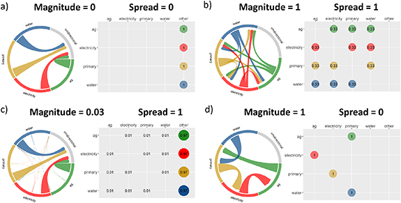
Figure 2. Examples showing the theoretical ranges of the 'Interconnectivity Magnitude Index' (Magnitude) and the 'Interconnectivity Spread Index' (Spread), selected to highlight the different information conveyed by the two indices. In each figure the chord diagrams are a visual representation of flows between sectors while the accompanying matrices show the share of each resource flowing from the sector in each row to the other sectors in each column. In each chord diagram, colored sectors are 'feedback' sectors, while gray represents a single lumped unidirectional 'other' sector. (a) 'Magnitude' = 0, 'Spread' = 0 (b). 'Magnitude' = 1, 'Spread' = 1 (c) 'Magnitude' = 0.03 and 'Spread' = 1. (d) 'Magnitude' = 1 and 'Spread' = 0. Regions experiencing high magnitude and high spread (e.g. figure 2(b)) are the most likely to benefit from multi-sector coordination.
Download figure:
Standard image High-resolution imageThe 'Interconnectivity Magnitude Index' (Magnitude) is a modified form of the 'network density' parameter as used in graph theory [65–68]. Network density is a simple quantification of the ratio of the number of actual connections in a network to the maximum possible number of connections. Using this network density concept, the 'Magnitude' index represents the ratio of the actual share of resources flowing to 'feedback sectors', as defined previously, to the maximum possible share of resources that can flow to 'feedback sectors'. This is represented mathematically in equation (1), where a share is calculated for each 'feedback sector', and then the mean value across all the sectors determines the final representative value of 'Magnitude'. The index is meant to be intuitive, with '0' indicating no resources are flowing to any 'feedback sector', and '1' indicating that all resources used in the region are flowing along paths connecting 'feedback sectors':
where:  'Interconnectivity Magnitude Index' (Magnitude)
 Number of feedback sectors
 Resource flows from feedback sector
  to feedback sector
 Resource flows from sector
  to 'Unidirectional sectors'.
While the 'Magnitude' quantifies the share of resources flowing to the 'feedback sectors' relative to 'unidirectional sectors', it does not indicate how widely the resources are spread across sectors. The Interconnectivity Spread Index (Spread) does precisely this. The 'Spread' is calculated based on a modified version of the root mean square error (RMSE) [69] to capture the deviation from a 'perfect spread'. The 'Spread' is designed to be intuitive, in the sense that '0' represents no spread, wherein resource flows are concentrated in only one of the 'feedback sectors'; and '1' represents the perfect spread, wherein resources are equally shared across all of the 'feedback sectors'. This is represented mathematically in equation (2), which calculates the squares of the differences between the actual shares across the total number (n) of 'feedback sectors' and the ideal shares representing the perfect spread (1/n). The difference is then normalized so that the maximum difference from the perfect spread results in a '0', while the minimum difference results in a '1':
where:  'Interconnectivity Spread Index' (Spread)
 Feedback sectors
 Resource flows from sector
  to sector
  .
.
The indices, as calculated in equations (1) and (2), are calculated for the United States for multiple scenarios based on the outputs of the GCAM-USA model [70, 71]. Analysis is conducted at both the National and State levels at 5 year time step intervals from 2015 to 2100, with 2015 representing a historical base-year. The scenarios define various representative socioeconomic and technological pathways in response to exogenously defined population, GDP, and emissions constraints, which in turn drive energy–water–land dynamics in GCAM-USA. We first run a Reference scenario ('Reference') to define baseline conditions against which to compare subsequent scenarios [3, 81–83]. Subsequent scenarios use the same basic assumptions built into the Reference scenario with regard to technologies advancement pathways, price and income elasticities, costs and resource availabilities. In addition to the Reference scenario, three additional scenarios ('Low Pop/GDP', 'High Pop/GDP', and 'Low Carbon') are also run to explore the implications of changes in population, GDP, and a low carbon future consistent with the representative concentration pathway (RCP) 2.6 [84, 85] (See SI2 for details on national and state population and GDP projections for each scenario). Key assumptions for each of the scenarios are summarized below and in table 1:
- Reference: The baseline assumptions that define the Reference scenario. These assumptions are also applied to all subsequent scenarios (with some modifications, as described in subsequent scenario descriptions). The Reference scenario assumptions are consistent with the shared socioeconomic pathway 2 (SSP2) for the world. The SSP2 scenario represents costs, prices, elasticities, and preferences in a 'middle-of-the-road' narrative in which social, economic, and technological trends do not shift markedly from historical patterns [3, 81, 82]. In the US, this scenario assumes a continuation of existing trends across systems in the near term, with economic forces driving changes in the longer term. Electricity demands are projected to increase in response to industrial electrification, while electricity supply is expected to see increasing shares of natural gas and renewable energy. In addition, both mature crude oil refining technologies as well as relatively immature and nascent technologies such as biomass to liquids, coal to liquids, and gas to liquids, are projected to expand to meet growing demands for liquid fuels (See further details in official documentation [71]). Population in the US increases to about 450 million and GDP to about $75 trillion (2015 USD) by 2100.
- Low Pop/GDP: All assumptions except for population and GDP in the US remain the same as in the Reference scenario listed previously. In this scenario, the population and GDP projections for the US are based on SSP3 [81, 86]. US population decreases to about 250 million in 2100 and GDP stays flat throughout the century at about $30 trillion (2015 USD) in 2100.
- High Pop/GDP: All assumptions except for population and GDP in the US remain the same as in the Reference scenario listed previously. In this scenario, the population and GDP projections for the US are based on SSP5 [81, 86]. US population increases to about 700 million in 2100 and GDP increases to about $275 trillion (2015 USD) in 2100.
- Low Carbon: All assumptions remain the same as in the Reference scenario listed previously, with the addition of a carbon tax to investigate the implications of a low carbon future consistent with representative concentration pathway (RCP) 2.6. While the Reference scenario leads to a radiative forcing of about 6 W m−2 in 2100, the 'Low Carbon' scenario results in a radiative forcing of 2.6 W m−2, leading to a 2 °C increase in mean global temperature relative to pre-industrial conditions (1850–1900) [87]. The lower emissions are enforced in GCAM-USA by applying an escalating carbon price that begins at $25/tCO2 (2010 USD) in 2025 and increases (at 5% annually) to about $1000/tCO2 (2010 USD) in 2100. These prices are consistent with the range of carbon prices (15–360 $/tCO2 in 2030 to 140–8300 $/tCO2 in 2100) used in various multi-model exercises [87, 88] for a representative concentration pathway of RCP 2.6 [84, 85].
Table 1. Summary of key differences between scenarios.
| Scenario name | Pop in year 2100 | GDP in year 2100 | Carbon tax starting in year 2025 |
|---|---|---|---|
| Reference | 450 million (SSP2) | $75 trillion (SSP2) | $0/tCO2 |
| Low Pop/GDP | 250 million (SSP3) | $30 trillion (SSP3) | $0/tCO2 |
| High Pop/GDP | 700 million (SSP5) | $275 trillion (SSP5) | $0/tCO2 |
| Low Carbon | 450 million (SSP2) | $75 trillion (SSP2) | $25/tCO2 (Increasing 5% annually to 2100) |
3. Results
3.1. National analysis
A core focus of this paper is to understand how interconnectivity may change in the future in the US under various scenarios that capture changes in population, GDP and technological shifts in response to a Low Carbon future. Figure 3(a) shows the evolution of the interconnectivity indices ('Magnitude' and 'Spread') in the US under the Reference scenario. We begin analysis at the national scale before progressing to finer-scale state-level analysis. At the national scale, the 'Magnitude' index remains relatively unchanged over time, showing only a slight decrease from 0.24 to 0.23 by 2100. This is because, at the aggregate national scale, the share of resources used within feedback loops relative to the share of resources used directly by end-users (in unidirectional flows) changes only very slightly over time and since the Magnitude Index is defined by this ratio it also shows a small change (see SI5 for exact numbers on the changes in these ratios for each scenario from 2015 to 2100). The small shifts in the index become more pronounced as we zoom into finer spatial scales (from national to states) as discussed later. The 'Spread' index moderately increases from 0.35 in 2015 to 0.39 in 2020 as a result of agricultural land being shared amongst new 'feedback sectors' (e.g. biomass for electricity as well as for primary energy). Agricultural land dedicated to purpose-grown biomass is introduced into the model in 2020 (0 km2 in 2015), with 1600 km2 used to produce biomass for electricity production and 14,000 km2 for liquid biofuels (out of a total of 1 million km2 of national agricultural land), thus increasing the Spread index nationally. The subsequent decline in the Spread index over time is primarily driven by a larger share of water withdrawals going towards the agricultural sector, as the power system becomes more water efficient by the end of the century (See SI3 and SI5 for further details on the evolution of the interconnectivity indices by sector).
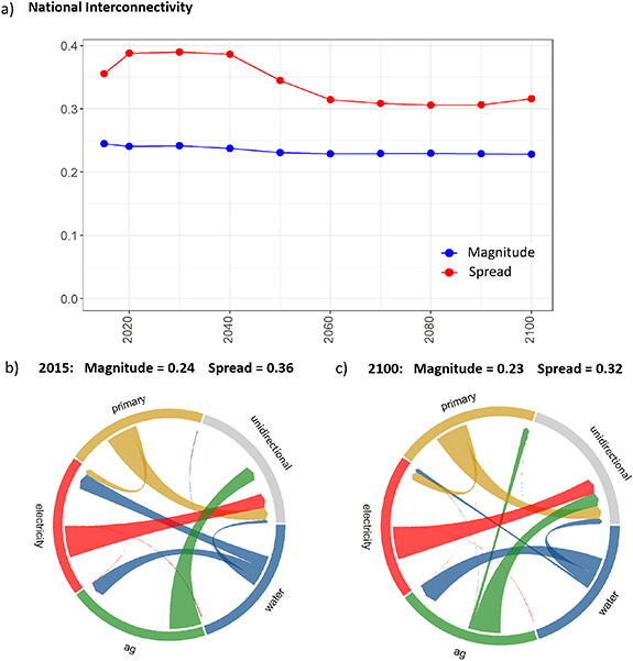
Figure 3. National interconnectivity for the United States in the Reference scenario. (a) Interconnectivity indices 'Magnitude' and 'Spread' from 2015 to 2100; (b) intersectoral resource share flows for 2015; and (c) intersectoral resource share flows for 2100.
Download figure:
Standard image High-resolution imageTo better understand how the composition of the two indices is changing over time, figures 3(b) and (c) show the makeup of intersectoral flows in 2015 and 2100, respectively. In 2015, sectoral interconnectivity is driven by water used for agriculture and electricity generation. Comparing figures 3(b) and (c) we can see a decoupling of the sectors, as water shifts away from electricity generation. This is explained by a shift in power plant cooling technologies from once-through cooling to more efficient closed-loop cooling, consistent with the SSP2 storyline (SI4). Additionally, results show an increase in agriculture flows to primary energy, which reflects the increase in purpose-grown biomass. The increasing water efficiency of power generation, and the use of agriculture in energy production, have opposite effects on the interconnectivity indices over time. Water shifting out of the 'feedback sectors' (from electricity to unidirectional sectors) decreases interconnectivity, while more agricultural land used for electricity and primary energy increases interdependencies between the 'feedback sectors'. Land use for purpose grown biomass expands into pasture, grass and other land and is unevenly distributed across the states (See SI4 for details on land use changes and its spatial distribution). The potential for multiple forces to counteract one another's impact on interconnectivity over time underscores the importance of evaluating the implications of multiple time-evolving human and earth system influences.
Figure 4 shows the effect of changes in population, GDP, and carbon constraints on interconnectivity. Relative to the Reference scenario, the 'High Pop/GDP' scenario shows a decrease in the Magnitude of interconnectivity but an increase in the Spread of interconnectivity. This is primarily driven by an increase in the share of water needs for municipalities and other unidirectional uses from 39% in the Reference to 56% in the High Pop/GDP scenario and with the relative share of water used for agriculture declining from 53% in the Reference to 35% in the High Pop/GDP scenario (See SI5 for chord diagrams and matrices). This shift is reflected by a decline in the Magnitude Index from 0.23 for the Reference scenario to 0.18 in the High Pop/GDP scenario. The shares of water used for agriculture (decreasing from 53% in the Reference to 35% in the High Pop/GDP scenario) and for electricity generation (increasing from 7% in the Reference to 9% in the High Pop/GDP scenario), however, become more balanced and are reflected by the increase in the Spread Index (from 0.32 in the Reference to 0.34 in the High Pop/GDP). In the Low Pop/GDP scenario we see the opposite effect: a larger share of water is used for agriculture, thus increasing the magnitude of interconnectivity but decreasing its spread across sectors as water becomes more concentrated in one sector. In the 'Low Carbon' scenario, purpose-grown bioenergy becomes more profitable and causes an increase in the magnitude of interconnectivity. This diversion of agricultural commodities into the energy sector strengthens the coupling of water, agriculture, and energy. The spread of resources across the 'feedback sectors' however declines as the share of water concentrates in the agriculture sector (See SI5 for the corresponding chord diagrams and matrices).

Figure 4. Absolute (top row) and % difference from Reference scenario (bottom row) for two national interconnectivity indices, 'Magnitude' and 'Spread', for all scenarios from 2015 to 2100.
Download figure:
Standard image High-resolution image3.2. Subnational (state-level) analysis
While figures 3 and 4 are useful for understanding general trends at the national level, many of the most important intersectoral conflicts, tradeoffs, and planning issues take place at the finer spatial scales. Accordingly, figure 5 telescopes down to the state level. The overall patterns seen in the national interconnectivity results are also observed at the state level with regard to the general character of the 'Magnitude' and 'Spread' trends across scenarios over time. However, some additional insights appear in the state level results that were not visible in the national results. For example, the Magnitude interconnectivity index is highest in the Reference scenario in the central states as shown in figure 5, driven by a higher fraction of their water being used for agriculture (See SI4 for the distribution of water use by sector and state). By 2100, eastern and western states show a drop in the Magnitude Index (See SI6 for details on changes in the spatial distribution of interconnectivity in the 'Reference' scenario from 2015 to 2100) as water is diverted away from 'feedback sector' cycles (agriculture, electricity and primary) towards direct end-use by 'unidirectional sectors' (such as industry and municipalities), while central states do the opposite (See SI4.4 for changes in the share of water across the states from 2015 to 2100). In eastern states the drop in the Magnitude Index is driven by the proportion of water used for powerplants decreasing, while in the western states the decrease is as a result of the proportion of water for agriculture decreasing. We see the opposite impact on the spread of resources ('Spread') amongst 'feedback sectors' in these same states.
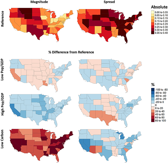
Figure 5. Distribution of 'Magnitude' and 'Spread' across states. Top map shows absolute values for the 'Reference' in 2100. Bottom three maps show the % difference from the 'Reference' scenario for the Low Pop/GDP, High Pop/GDP and Low Carbon scenarios in 2100.
Download figure:
Standard image High-resolution imagePurpose-grown biomass becoming more competitive in the 'Low Carbon' scenario results in an increase in the coupling of sectors, as more biomass is grown across states. East and west coast states show the highest increases corresponding to the shift in land use for biomass (SI4). In the 'High Pop/GDP' scenario, we again see a decoupling of sectors (drop in the Magnitude Index) across the US, driven by a larger proportion of water used directly by municipalities as compared to agriculture or electricity. This decoupling is most pronounced in the states with the highest increases in population such as California (SI2). On the other hand, we see an increase in the Spread Index in several states primarily driven by a relatively more equal distribution of water use for power plant cooling and agriculture (SI5). For the case with a decline in population and GDP (Low Pop/GDP), we see an increase in sectoral interconnectivity, as more resources are used within processes that share resources as compared to unidirectional flows to end uses, but a decrease in the spread as resources become concentrated in particular sectors.
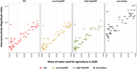
Overall, the share of water used for agriculture use (figure 6) shows the strongest correlation with the Magnitude Index across the states from amongst the parameters analyzed in this study (See SI8 for additional charts showing Interconnectivity Indices vs changes in various parameters). The Spread Index on the other hand does not show any particularly strong correlation with any of the parameters considered. This result holds across scenarios with an overall increase in coupling in the case of the 'Low Carbon' scenario as a result of additional water needed for purpose-grown biomass.
Figure 6. Interconnectivity Magnitude Index values vs share of water used by agriculture for all states and scenarios in 2100.
Download figure:
Standard image High-resolution image
4. Discussion
The results from figures 3–6 complement analysis of indirect impacts from other studies calling for the co-management of resources and provide additional insights into how those interactions may change in the future. Brown et al [26] identifies most of the southwest and lower midwest basins in the United States to be at risk of monthly water shortages during the period from 2049 to 2070. A deeper look into the interconnectivity indices of some of these states (SI6 and SI7) highlights some of the dynamics at play and provides insight into how similar levels of water shortages in different basins could benefit from different multi-sector co-management approaches (SI9). States like Colorado (CO) and Kansas (KS) show the highest combined interconnectivity parameters (both 'Magnitude' and 'Spread' higher than 0.25 in 2100), and in both cases the highest share of water is used by agriculture from 2015 to 2100. In other states like Arizona (AZ) with similar projections for water scarcity, the 'Magnitude' index is lower, and the distribution of resources shows that water stress will need to be managed by coordinating between the water and electricity sectors. In New Mexico (NM), we see a large increase in the concentration of the share of agriculture grown for electricity, with purpose-grown biomass increasing from 0% in 2015 to 30% in 2100. This comes with a corresponding increase in water for agriculture (from 70% in 2015 to 80% in 2100) and a reduction in the share of water used for power plant cooling. In the 'Low Carbon' scenario, these numbers increase even more, with 85% of agriculture used for biomass for electricity, and the share of water for agriculture increasing to almost 90%. In the face of severe water shortages, these results indicate that strategic co-management of land, water resources, and electricity production could produce benefits.
The Fourth National Climate Assessment [6] highlights California as a key example of a region with critical interconnectivity among water, energy, and agricultural resources. The water system is the largest single electricity user in the state (3% of total), agriculture is the largest water user, and a substantial amount of electricity is generated using hydropower. Our results show how these intersectoral dynamics could shift in the future. Our results show that a larger population (High Pop/GDP scenario) could decouple local resources, with a significantly larger share of water being used directly for industries and municipalities ('Unidirectional' sectors) instead of agriculture by 2100 (figure 5). Remaining resources (in this case primarily water), however, are more equally shared across the 'feedback sectors', indicating a greater need for co-management to distribute shared resources efficiently to meet multiple objectives.
The US Energy Information Administration (EIA) [89] analyzes the distribution and decline in water intensity of US powerplants. The largest quantities of water for powerplant cooling are withdrawn in the eastern half of the country [28, 29]. This distribution is also reflected in the 'Spread' map (figure 5), where water is shared more equally between agriculture and powerplants. Our results also show a decline in water and electricity coupling as a result of more efficient powerplant cooling to 2100. Voisin et al [33] and van Vliet et al [90] showed high vulnerability of the power system to water temperature and availability. In the western US, the electricity grid was shown to have a 21% chance of insufficient generation based on 30 years of historical water availability data simulations [33]. The combination of our 'Magnitude' and 'Spread' maps with state level chord diagrams show a trend of water being shared more equally between agriculture and electricity in the eastern half of the country as compared to the west, where water use is dominated by agriculture (See SI4). These reflect important implications for how water shortages will be managed between resources in the future, with the share of allocations and water rights possibly indicating sectoral clout when it comes to decision making.
The results in figures 4 and 5 comparing the changes in the indices across the scenarios showed that the sectoral interconnectivity ('Magnitude') increased the most in the Low Carbon scenario driven by biomass production for primary energy liquid biofuels (with a 60% increase in 'Magnitude' by 2100 for 'Low Carbon' scenario) and corresponding increases in water for energy. These results complement previous studies exploring the emission implications of bioenergy production [91, 92] and weighing the benefits against cross-sectoral impacts on water and land [43].
5. Conclusions
Interdependency between water, energy, agriculture, and other sectors results in indirect impacts, wherein changes in resource availability and demands in one sector have the potential to propagate across multiple sectors in nonlinear and unexpected ways [6]. Several studies have documented examples of these indirect impacts and cascading effects [8, 11, 16, 48, 49, 57–64]. The various linkages among sectors via physical commodity flows have also been well documented, such as water needs for power plant cooling, water for agriculture, biomass for energy, and electricity for water processing [5–23]. An understanding of these interdependencies can help planners to capitalize on synergies as well as avoid trade-offs. This paper complements previous studies that focus on measuring the impacts of interconnectivity by explicitly quantifying and visualizing the interconnectivity itself and how it varies across space and time. It does so by first classifying 'feedback sectors' as those sectors which form part of feedback loops. Indices are then defined to quantify the share of resources flowing through these feedback loops as well as to quantify to what degree resources are shared between the 'feedback sectors'. This approach can be applied to understand the potential evolution of interconnectivity over time, as well as to identify regions that might benefit most from coordinated co-management of resources. While we apply this novel methodology in a US context, the methodology can flexibly be applied in diverse geographic and sectoral contexts.
In this case study for the US, results show that coupling between sectors is primarily driven by water used for agriculture and powerplant cooling. The results for the Reference scenario show a decoupling of sectors nationally over time, from 2015 to 2100, as the power system becomes more water efficient with shifts from once-through power plant cooling to more efficient recirculating cooling. This releases a significant amount of water from the power sector, which used 40% of total US water withdrawals in 2015, to 7% in 2100. At the same time, an increase in purpose-grown biomass (from 0% of all agricultural land in 2015 to 10% in 2100) contributes to increasing intersectoral connectivity between water, agriculture, and energy.
While it could potentially be valuable to evaluate interconnectivity at the national scale for purposes of strategic planning, many of the most important intersectoral conflicts, tradeoffs, and planning issues take place at the state, county, and municipal scales. As we telescope from national scale to state-level spatial scale, sectors become increasingly decoupled as resource usage concentrates into fewer sectors. The emergence of regionally differentiated interconnectivity trajectories underscores the importance of the flexibility of the methodology we introduce to explore interconnectivity across diverse spatial scales. Subnational results across the states show that the highest sectoral interconnectivity is concentrated in the central states, with high relative use of water for agriculture and electricity as compared to other uses. Projected changes in interconnectivity across the states over time depend on the evolution of the power and land use systems. Along the east coast, our results project a decoupling of sectors due to a shift toward more water-efficient power plants. Meanwhile, along the west coast, the primary driver of decoupling is a decrease in the share of water used for agriculture. Increases in population and GDP (High Pop/GDP scenario) were seen to decouple systems by diverting resources out of feedback loops and into direct use by municipalities and industries, while the opposite was true for decreasing populations and GDP. A scenario exploring a Low Carbon future showed an increase in interconnectivity as a result of the expansion of purpose-grown biomass and a corresponding increase in the sharing of resources between water, agriculture, and energy. The scenarios we explored demonstrate the potential for multiple forces to counteract one another's impact on interconnectivity over time, thus underscoring the importance of evaluating the implications of multiple time-evolving human and earth system influences.
Broadly, the results of this study complement previous studies that have identified sector-specific hotspots (water scarcity, biomass expansion, technology advancements). For example, some regions of the world may be projected to become water scarcity hotspots in the future [25]. However, this does not explicitly offer insight into the complex web of sectoral interconnections that may be driving water scarcity in particular regions. In some regions, the solutions to water scarcity might be resolved by better management of water resources in limited sectoral certain contexts, such as irrigation efficiency. However, in other regions, water scarcity may be the result of complex multi-sector interconnections that will require more complex management strategies and coordination to resolve. In other words, increasing water (or other resource) scarcity alone does not imply a more complex co-management challenge. To improve insight into the multi-sector dynamics that may cause particular sectoral challenges to emerge in the future, here we introduce an approach to characterizing connectivity with novel indices. These indices, and future extensions of them, have the potential to provide a more holistic perspective regarding where multi-sector hotspots might emerge in the future, and which regions would benefit from coordinated, multi-sector co-management of resources to alleviate these sectoral challenges.
This study has several limitations that could be addressed in future work. The choice of the 'feedback sectors' used here was based on the identification of multi-directional flows of physical commodities between sectors. In the current study, in order to simplify the analysis, we did not consider some potential resource flows, such as waste products returning to the system, and various other segments of the industrial sector which are water and energy intensive such as fertilizer, cement, iron, steel, desalination, refineries, and petrochemicals. Taking on the industrial sector would require additional efforts on the GCAM front, thus, we decided to investigate additional levels of sectoral disaggregation such as fertilizer in future studies. Additionally, water withdrawals were used to calculate the interconnectivity in the water sector, instead of water consumption. Using water consumption instead of water withdrawals in the calculation of the indices would result in significantly different trends, since as power plants become more water efficient, they withdraw less water but consume more water. The results for the interconnectivity indices using water consumption are provided in SI10 and the largest difference is that because water consumption is concentrated in the agricultural sector in the US, the spread index is considerably lower. Several of the resource share calculations, such as electricity used for water processing (of surface water, groundwater, and desalinated water) and agriculture, were based on static coefficients from 2015 US values. Thus, technological advancement in those sectors are not captured, unlike how we capture power plant water efficiency improvements over time. In those cases, for example for electricity for water, the value of electricity increases in proportion to the increase in water withdrawn from surface water, groundwater, and desalinated water. This, however, is a limitation of the model used to calculate the distribution of resources (i.e. GCAM-USA in this case). We note that the interconnectivity indices as calculated in this study reflect the various human and Earth system assumptions as well as the management decisions made in each scenario for the various resources as portrayed by the underlying model. An exploration of these underlying decisions and the drivers behind them are beyond the scope of the current study and will be investigated in more detail in future studies.
A large body of research literature has confirmed the importance of understanding interdependencies between sectors to capitalize on intersectoral synergies and avoid cascading trade-offs. This paper introduces a new methodology to explicitly visualize and quantify the interconnectivity between resources. The results highlight that while some regions may have similar sectoral resources stress projections, the composition of the intersectoral connectivity that leads to that sectoral stress may call for distinctly different co-management strategies. This methodology, and any future extensions of it, will allow planners to better understand where, when, and how coupling or decoupling between sectors will evolve. Ultimately, this can lead to efficient, resilient systems that are more capable of handling multiple stressors across sectors.
Acknowledgments
This research was supported by the US Department of Energy, Office of Science, as part of research in MultiSector Dynamics, Earth and Environmental System Modeling Program. The Pacific Northwest National Laboratory is operated for DOE by Battelle Memorial Institute under contract DE-AC05-76RL01830. The views and opinions expressed in this paper are those of the authors alone.
Data availability statement
The data that support the findings of this study are openly available at the following URL/DOI: https://github.com/zarrarkhan/khan_et_al_2021_interconnectivity_usa.